Naive Bayes §

• Deep Learning Foundations and Concepts

Naive Bayes is a simple but powerful algorithm often used for text categorization, including spam filters. A Naive Bayes spam filter correlates the words in an email with spam and non-spam emails to determine the probability of the email in question being spam.

The algorithm is called “naive” because it treats all word orders the same. For instance, applied to spam email classification, Naive Bayes ignore grammar rules and common phrases: it treat texts as they’re just a bag full of words. (Keeping track of every single grammar rule is impossible ofcourse). Even though, it still works for spam classification.

Naive Bayes Definition §

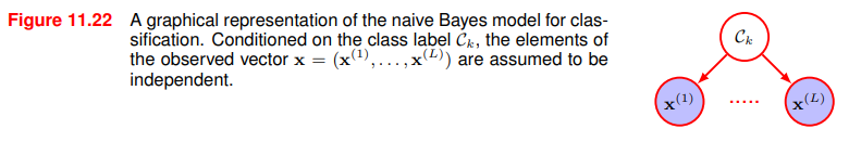
Formally suppose our data consists of observations of a vector of words and we wish to assign each values of to one of the two classess (“spam”, “not spam”).

We can define the class-conditional density for each of the classess: and , along with prior probability .

The key assumption of the Naive model is that, conditioned on the class , the distribution of the input variable factorizes into the product of two or more densities.

Suppose we partition into elements , Naive Bayes takes the form:

Note that, this assumption is generally not true but simplify the estimation dramatically:

• the individual class-conditional marginal densities can each be estimated separetly using one-dimensional kernel density estimates. The original naive Bayes procedures used univariate Gaussians to represent these marginals

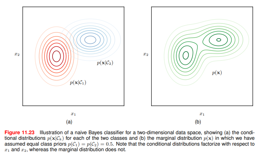
The figure shows that and are conditionally independent, which is the key “naive” assumption of this model.

If we are given a labelled training set with their class label, we can train a classifier using MLE, assuming that data are drawn independently from the model.

The solution is obtained by fitting the model for each class separately using the corresponding labelled data and then setting the class priors equal to the fraction of training data points in each class.

Then, the probability that a vector belongs to class is then given by Bayes’ theorem in the form:

We defined previously, and can be defined as: .

Putting the definitions into the bayes theorem:

In general for partitions of the training data and classes (with dataset labelled according to these classes).

For two classes (like email spam detection), we can write:

with marginal density given by:

Unfortunately, is a mixture of Gaussians and does not factorize wr.t. and .

When it is useful §

When the dimensionality of the input space is high, making density estimation in the full -dimensional space more challenging.

It is also useful if the input vector contains both discrete and continuos variables, since each can be represented separately using appropriate models e.g. Bernoulli for binary observations or Gaussians for real-valued variables.

Gaussian NB is just a way to say approximate conditional probability with univariate gaussian density.

Links §

• Naive Bayes is often explained under the Graphical Models by Bishop

Pratical Laboratory: Naive Bayes from scratch §

For this part i’ll skip data visualization and i’ll focus on implementing from scratch the naive bayes and then testing error.

Consider the well known heart.csv dataset that contains cardiac features of patients. Some features that have affect on heart like age, gender, blood plessure, cholesterol levels, ECG and so on.

from google.colab import drive
import pandas as pd
import numpy as np
import os

file_path = "/content/drive/MyDrive/MyLabs/NaiveBayesClassifier/heart.csv"

data = pd.read_csv(file_path) # for simplicity i'll skip testing the file

One of the feature is “target”, 1 if the patient has ad an heart attack, 0 otherwise.

y= data['target']
X=data.drop('target',axis=1)
 
# Create train and test dataset
from sklearn.model_selection import train_test_split
X_train, X_test, y_train, y_test = train_test_split(X, y, test_size=0.25, random_state=42, shuffle=True)
 
# Compute mean and std for each feature
mean = X_train.mean()
std = X_train.std()

To estimate the conditional probability, we need to define a density function. Gaussian i.e normal is usually a good enough approximation for this simple case

def density_function(X, mean, std):
  density = (1 / np.sqrt(2 * np.pi * std**2)) * np.exp(-((X - mean)**2) / (2 * std**2)) # Gaussian
  return density

Now let’s define a prediction function.

classes = np.unique(y.tain) #Classes are either 1 or 0, so two
predictions_per_class = [] # At the end we will have 2 items in this list

for c in classes:
	# Compute prior probability for the class
	prior_prob_class = np.sum(y_train==c)/len(y_train)
	
	# Filter X_train for the current class
    Xc = X_train[y_train == c]

• y_train==c means in the first case use y_train = 0 and in the second iteration y_train = 1
• We also consider only the subset of data () that has .

for c in classes
	...
	# Calculate mean and std for each feature within the current class
    mean_class = Xc.mean()
    std_class = Xc.std()
    
    # Add a small epsilon to standard deviation to avoid division by zero
    std_class = std_class.replace(0, 1e-6)

Machine Learning is deeply rooted in practice and empirical. We need to consider adjustation that avoid division by zero, in this case adding a small value .

Mean and standard deviation will be used for density: . Given the mean and standard deviation across the entire dataset, we can feed it to the previously defined density function. So thanks to these three information: mean, std and a data point, we can compute an approximation of the conditional probability for a given class .

So from the bayes formula:

Until now we have the prior probability and the conditional probability for a single point.

But we have said that naive bayes takes the form: and so:

Therefore the density function have to be applied to each point

for c in classes:
	...
	likelihood_class = 1.0
	
    # Iterate over actual feature names (columns) of the observation
    for feature in X_observation.index:
	    density = density_function(X_observation[feature], mean_class[feature], std_class[feature])
	    likelihood_class *=density

• this piece of code is the exact translation of where is the number of features for each data point .

Then we compute the unnormalized posterior probability:

for c in classes:
	...
	# Compute posterior probability (unnormalized)
	predictions_per_class[c] = prior_prob_class * likelihood_class

That is:

I would like to normalize it, even if the code also works without normalization:

# outside the "for c in classes loop"
total_prob = sum(predictions_per_classes.values())

# Normalize
for c in classes:
	predictions_per_classes[c] /= total_prob

Now we have:

predicted_class = max(predictions_per_class, key=predictions_per_class.get)
return predicted_class

Apply the Bayes classification criteria i.e assign the datapoint to the class with the maximum posterior probability.

Now, we can verify the results. Apply the prediction function to each data point of the training set:

predictions = []
for i in range(len(X_test)):
    # Get a single observation (row) from X_test
    X_observation = X_test.iloc[i]
    predicted_class = pred_function(X_observation, X_train, y_train)
    predictions.append(int(predicted_class))

print("Predictions for X_test:")
print(predictions)
print(f"Number of predictions: {len(predictions)}")

As metric for this toy example we’ll use accuracy, so:

accuracy = np.mean(predictions == y_test)
print(f"Accuracy: {accuracy}")

error_rate = 1 - accuracy
print(f"Error rate: {error_rate}")

Which evaluates to:

Accuracy: 0.881578947368421
Error rate: 0.11842105263157898

More rigorous test should be done using cross-validation. Notice how the accuracy lowers when we consider the entire dataset:

# Evaluate the model on the entire dataset
y_pred =[]
for i in range(len(X)):
  X_obs = X.iloc[i]
  pred = pred_function(X_obs, X_train, y_train)
  y_pred.append(int(pred))


accuracy = np.mean(y_pred == y)
error_rate = 1 - accuracy
print(f"Accuracy: {accuracy}")
print(f"Error rate: {error_rate}")

Output:

Accuracy: 0.8283828382838284
Error rate: 0.17161716171617158

---