Hypothesis Testing and p-values, chi2 , permutation, likelihood ratio test, multiple testing and goodness-of-fit testing

---

Hypothesis Testing and p-values

• Source textbook: “All of statistics” Chapter 10

Suppose we want to know if exposure to asbestos (a desease) is associated with lung disease. We take some rats and randomly divide them into two groups. One is eposed to asbestos and the second group is unexposed. Then we compare the disease rate in the two groups.

Null Hypothesis

The null hypothesis: the disease rate is the same in the two groups The alternative hypothesis: the disease rate is not the same in the two groups.

If the exposed group has a much higher rate of diesease than the unexposed group then we will reject the null hypothesis annd conclude that the evidence favors the alternative hypothesis.

Suppose that we partition the parameter space into two djsoint sets and and that we wish to test:

We call the null hypothesis and the alternative hypothesis.

Hypothesis testing

Let be a random variable and let be the range of . We test a hypothesis by finding an appropriate subset of outcomes called the rejection region.

• reject
• retain

Usually the rejection region R is of the form:

• is a test statistic
• is a critical value.

The problem in hypothesis testing is to find an appropriate test statistic and an appropriate critical value .

Warning: hypothesis testing methods are appropriate only when there is a well-defined hypothesis. Otherwise use estimation or confidence intervals.

Intuition: Hypothesis testing is like a legal trial. We assume someone is innocent unless the evidence strongly suggets that he is guilty. Similarly we retain unless there is strong evidence to reject .

Type of errors

• Type I error: rejecting when is true
• Type II error: retaining when is true

Definition: power function The power function of a test with rejection region is defined by:

The size of a test is defined by

A test is said to have level if its size is less than or equal to .

Simple vs composite hypothesis:

• A hypothesis of the form is called simple
• Otherwise if or is called a composite hypothesis

A test can be two-sided like:

or

is called a one-sided test.

The most common tests are two sided.

It would be desiderable to find the test with highest power under among all size of tests. Such a test, if it exists, is called most powerful. In practice this is hard and in many case it doesn’t even exists.

The Wald Test

Let be a scalar parameter, let be an estimate of . Let be the estimated standard error of .

Consider testing: versus Assume that is asymptotically Normal:

The size of Wald Test is: reject when where:

Theorem asymptotically the Wald test has size .

Alternative version:

• is the standard error computed at

Theorem: Suppose the true value of is . The power i.e the probability of correctly rejecting the null hypothesis is given (approximately) by:

Recall that tends to 0 as sample size increases.

Example: Comparing Two prediction Algorithms

Let be the size of the test set on which Algorithm 1 is tested. Algorithm 2 is tested on another test set of size Let be the number of incorrect prediction for A1 and Let be the number of incorrect predictions for A2. Let Binomial() and \Binomial(). The null hypothesis is so we can write versus where . The MLE is with estimated standard error: The size of Wald test is to reject when where: The power of this test will be largest when is far from and when the sample sizes are large.

Theorem: The size Wald test rejects versus if and only if where:

Thus, testing the hypothesis is equivalent to checking whether the null value is in the confidence interval.

The difference between statistical significance and scientific significance is easy to understand in light of previous theorem. Any confidence interval that excludes corresponds to rejectin . But the values in the interval could be close to (not scientifically significant) or far from ( scientifically significant)

p-Values

Rejecting or retaining an hypothesis is not very informative. Instead we could ask for every whether the test rejectrs at that level.

Generally, if the test rejects at level it will also reject at level : Hence there is a smallest at which the test rejects and we call this number the -value.

Definition: Suppose that for ever we have a size test with rejection region . Then:

That is the smallest level at which we can reject .

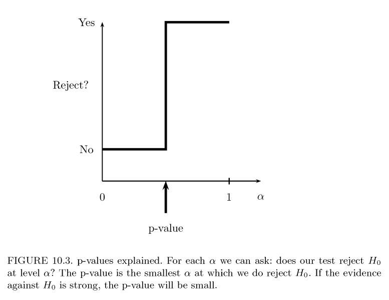
Informally, the p-value is a measure of evidence against : the smaller the p-value, the stronger the evidence against . Typically researchers use the following evidence scale:

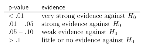
A large p-value is NOT strong evidence in favor of

A large p-value can occur for two reasons:

1. is true
2. is false but the test has low power

p-value IS NOT the probability that the null hypothesis is true

Theorem: suppose that the size test is of the form:

• reject if and only if

Then

• p-value =

where is the observed value of . If then:

• p-value =

We can express previous theorem as: “The p-value is the probability (under ) of observing a value of the test statistic the same as or more extreme than what was actually observed.”

Theorem Let denote the observed value of the Wald statistic . The p-value is given by:

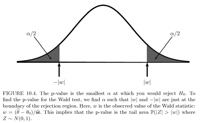
Theorem: if the test statistic has a continuos distribution, then under the p-value has a Uniform(0,1) distribution. Therefore rejecting when the p-value is less than , the probability of a type error is .

Intuition: In other words if is true, the p-value is like a random draw from a Uniform(0,1) distribution. If is ture, the distribution of the p-value will tend to concentrate closer to 0.

The ^2 Distribution

distibution

Let be independent, standard Normals.

Let .

We say that has a distribution with degrees of fredom, written as .

The probability density of is:

• for

It can be shown that and .

The upper quantile is

• where is the CDF
• that is

Pearson’s test for multinomial data

This test is used for multinomial data.

• The name is similar to Pearson Correlation Coefficient for Feature Selection

Recall that if has a multinomial distribution, then the MLE of is

Let be some fixed vector and suppose we want to test: versus

Definition: Pearson’s statistic is:

• where is the expected value of under

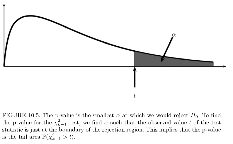
Theorem Under , . Hence the test: reject if has asymptotic level . The p-value is where is the observed value of the test statistic.

Example - Mendel’s peas

Mendel bred peas with round yellow seeds and wrinkled green seeds. There are four types of progeny: round yellow, wrinkled yellow, round green, and wrinkled green.

The number of each type is multinomial with probability . His theory of inheritance predicts that is equal to:

In trials he observed that .

We test that versus .

Since , , and , the test statistic is:

The value for is 7.815. Since we do not reject the null. The -value is: which is not evidence against . Hence the data do not contradict Mendel’s theory.

In the previous example, one could argue that hypothesis testing is not the right tool. Hypothesis testing is useful to see if there is evidence to reject but does not prove that is true. It might occur for example because the test has a low power.

Perhaps a confidence set for the distance between and might be more useful in this example.

Permutation Test

The permutation test is a nonparametric method for testing whether two distributions are the same.

This test is “exact,” meaning that it is not based on large sample theory approximations.

This is the kind of test to consider when testing whether a treatment differs from placebo.

Let and Let . The hypothesis is that the two distributions are identically distributed:

• versus

Let be some test statistic, for example:

Let and consider forming all permutations of the data. For each permutation, we compute the test statistic , denoting these values as .

Under the null hypothesis, each of these values is equally likely. The distribution that puts mass on each is called the permutation distribution of .

Let be the observed value of the test statistic. Assuming we reject when is large, the p-value is:

• is the indicator function

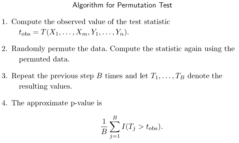
Algorithm for Permutation Test:

In large samples, the permutation test usually gives similar results to a test that is based on large sample theory. The permutation test is thus most useful for small samples.

The Likelihood Ratio Test

• See also: ML1 lec3/ML1 - Lec4

It can be used for vector-valued parameter

Consider testing:

The likelihood ratio statistic is:

It is most useful when consists of all parameter values such that some coordinates of are fied at particular values.

Goodness-of-fit Tests

It is used when we want to check whether data come from an assumed parametric model.

There are many such test, here is one.

Let be a parametric model. Suppose the data takes real values on a line. Divide this line into disjoint interval for let:

be the probability that an observation falls on under the assumed model.

Here are the parameters in the assumed model. Let be the number of observations that fall into . The likelihood for based on the counts is the mulinomial likelihood:

Maximizing yields estimate of .

Now define the test statistic:

Theorem let be the null hypothesis that the data are IID draws from the parametric model . Under , the statistic defined in previous equation converges in distribution to random variable. Thus the (approximate) p-value for the test is where denotes the observed value of .

Goodness-of-fit testing has some serious limitations. If we reject then we conclude that we should not use the model. But if we do NOT reject then we cannot conclude that the model is correct.

We may have failed to reject simply because the test did not have enough power. This is why it is better to use nonparametric methods whenever possible rather than relying on parametric assumptions.

Multiple Testing

In some situations we may conduct many hypothesis tests.

Multiple testing problem Suppose each test is conducted at level . For any one test, the chance of a false rejection of the null is . But the chance of at least one false rejection is much higher. This is called multiple testing problem.

The problem comes up in many data mining situations where one may end up testing thousands or even millions of hypotheses.

There are many ways to deal with this problem. Here we discuss two methods.

Consider hypothesis tests: versus with and let be the p-values for these tests.

Bonferroni Method

Given p-values , reject the null hypothesis if

Theorem: Using the Bonferroni method, the probability of falsely rejecting any null hypotheses is less than or equal to .

False Rate of Discovery (FDR)

The Bonferroni method is very conservative because it is trying to make it unlikely that you would make even one false rejection.

Sometimes, a more reasonable idea is to control the false discovery rate (FDR) which is defined as the mean of the number of false rejections divided by the number of rejections.

Suppose we reject all null hypothesis whose -values fall below some thresh-old. Let be the number of null hypothesis that are true and let . The tests can be categorized in a table.

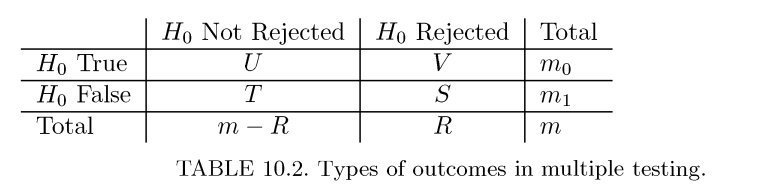
The False Discovery Proportion (FDP) is:

The FPD is the proportion of rejections that are incorrect. Next define EDR=.

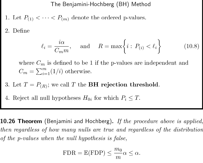
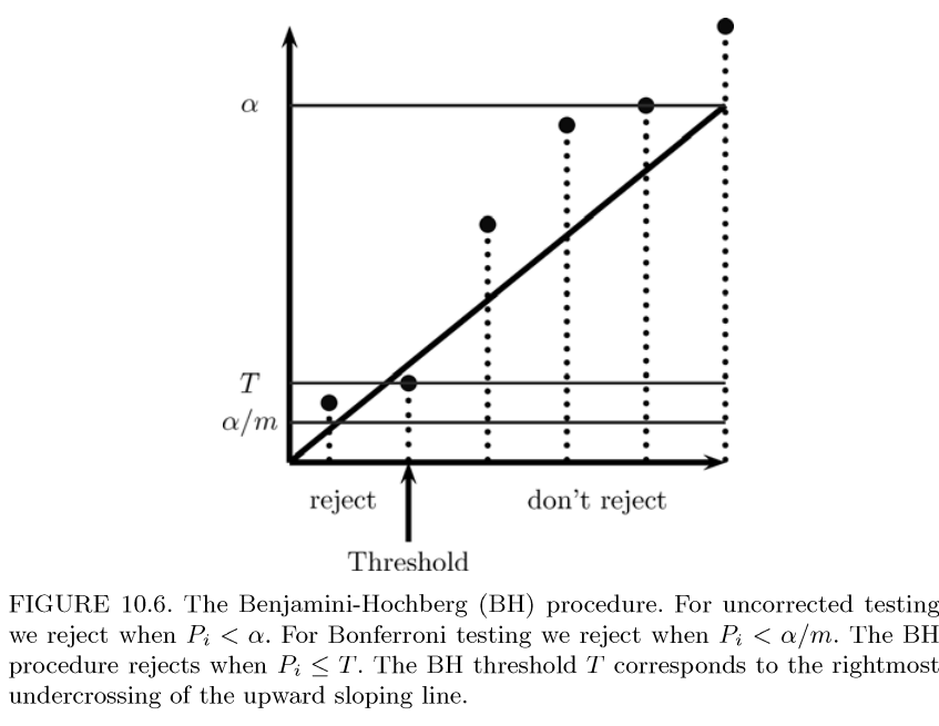
The Benjamini-Hochberg (BH) method