SC - Lezione 17 - Conjugate Gradient, Minimization Applications, Maximization of the Likelihood and Logistic Regression

---

SC - Lezione 17 §

---

Checklist §

Checklist

Domande, Keyword e Vocabulary §

• Conjugate Gradient
• symmetric matrix
• when it is better to use Conjugate Gradient respect to Gauss or LU?
• quadratic function
• Real world applications of minimization
• Nonlinear Least Squares exponential fitting
• Fitting of a nonlinear model
• Maximization of the likelihood
• Parameters of the gaussian distribution /normal function
• What is the Likelihood?
• Logistic Regression
• What is the Sigmoid Logistic Function??
• Medical dataset example
• Logistic Regression
• Binary classifier
• Bernoulli Probability
• Log-Likelihood
• Admission status - student exam scores example
• Robotic Arm

Appunti SC - Lezione 17 §

Conjugate Gradient §

(in green the optimal step size, in red the conjugate vector)

What it is used for §

To solve a linear system where is a symetric matrix. (therefore square)

As conseguence of the symmetry, the matrix S is positive definite, means that all its eigenvalues are positive numbers.

Approximation §

Unlike Gauss Method and LU Factorization methods which are direct methods for linear systems, CG generates a sequence of of approximations that converges, upon suitable coniditions, to the solution of the linear system.

Gauss Method vs LU method vs Conjugate Gradient §

Question: when it is better to use Conjugate Gradient respect to Gauss or LU? Answer: When the matrix is very large and sparse. Because, in order to compute each approximation, it will do a couple of matrix-vector multipication. If is sparse, the vector multiplication has a lesser cost.

So, the conjugate matrix can be very effective in this case. The very fast convergence of the conjugate gradient comes from this:

Quadratic Function §

Consider the quadratic function:

then

Therefore we can solve the problem of finding the minimum x of f(x) by solving the linear system

S-conjugate-norm of a vector If you take any vector, you can define a new norm that depends on the matrix S, called S norm such that: , and the so-called S-scalar product , so that if it happens that then the two vectors and are called S-orthogonal or conjugate.

Initial approximation and residual CG starts with an initial approximaton and the first residual is . Note that . The vector is the first search direction on which the next approximation is computed as where

is the scaled directional derivative of at in the direction . Notice that is scaled respect to the S-conjugate-norm

Second residual The second step is to compute that is residual defined as: There is a relationship between and since: and then in setting the new search direction where is defined in such a way that and are conjugate, that is and finally in computing the next approximation and so on.

Alternative quadratic functions §

We saw that CG can minimize quadratic functions of the form:

But it also works on more general quadratic functions of the form:

where the is a scalar.

Since , the scalar is deleted when you compute the derivative.

Second Derivative §

The second derivative of the quadratic function is constant since it coincides with the symmetric matrix.

Why it is efficient §

The CG method works well for minimization because it doesn’t merely follow the steepest gradient at each step (as in regular gradient descent). Instead, it uses a sequence of directions that are conjugate to each other relative to . This ensures that each step is independent of previous steps in terms of progress toward the solution.

The sequence of conjugate directions have the property of being -orthogonal (conjugate) with respect to the matrix , allowing for efficient minimization path.

Real-World Applications of Minimization §

Nonlinear Least Squares: exponential fitting §

The problem Minimization problem in which we are given a set of nodes and corresponding values , and we want to fit them into the following nonlinear model:

We want to solve the problem in the Least Square sense, that is:

The true parameters of the vectors are the one of the unperturbed model.

I want to minimize the 2 norm of this function that depends from c. We are not really interested in . The function has 5 variables which are unknown parameters of the fitting.

The true goal of this method is not to compute the exactly true line, the exponential with the true parameters choosen at the beginning (in the example):

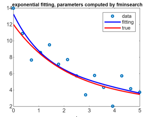
But we want to compute an approximation, a fitting that is the blue line

But we have seen other problem to solve this problem like a gradient descent method: 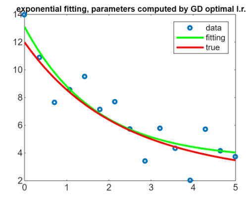And it also works really really well.

There are also some other matlab functions, one of these is called lsqcurvefit.

Maximization of the likelihood §

We want to maximize the likelihood of a dataset , with respect to the choice of the parameters of a Gaussian distribution from which such data were extracted. (Backlink a ML per la distribuzione gaussiana)

What is the likelihood §

The likelihood is a function that measures how well a statistical model explains observed data by calculating the probability of seeing that data under different parameter values of the model.

In our example, we consider a Gaussian distribution, so the likelihood depends on the two parameters: the mean and the variance ( and ).

We start with a set of data extracted from a Gaussian distribution with fixed mean and variance and try to recover the value of the mean and the value of the variance by maximizing the likelihood of the dataset.

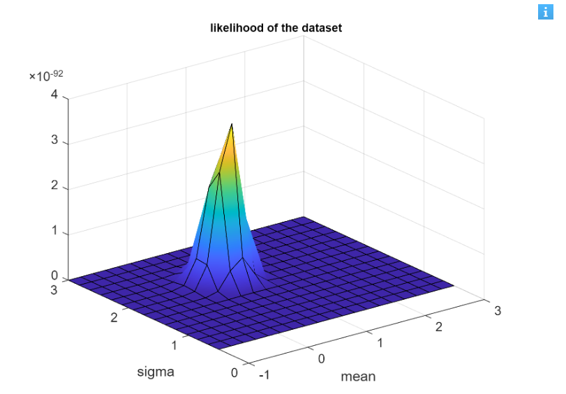As we can see this graph depends from three variables: sigma that is the variance, mean that is and on the z we have the output of f given the two parameters.

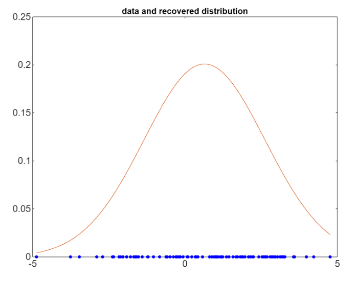To maximize the likelihood we look for the minimum of the negative of the likelihood function.

Logistic Regression and maximization of likelihood §

An application of the maximization of likelihood is the logistic regression, that is an important tool used in binary classification. (backlink a ML)

What is the Sigmoid Logistic Function? §

The sigmoid logistic function is a function, usually used often for describing population grows; initially very fast then it arravies at a stable point.

Description of the problem §

For instance, consider a medical dataset when you want to classify if a patient has flu or not, and you have set of parameters. We use the logistic regression to classify a new sample (a new patient), that does not belong from the starting dataset.

In general: Consider a dataset that consists of pairs of data points (features) and labels that gives us the interpretation of the i-th sample.

• has a value 1 or 0.

Note: The Logistic Regression is not a regression, even if the name may trick you. It’s a binary classifier.

You maximize the likelihood to compute the parameters of a model.

is the outcome of the linear model, and, are parameters of the model that must be computed during the training of the model.

By maximing the likelihood the training data we compute the parameters

Likelihood definition for this problem §

The probability that the model, given a set of parameters, produced the observed results. In our example we can express it as:

As Bernoulli distribution

If we call the set of parameters we can write:

Note: i called the set of parameter as B because i think it’s clearer, but it’s not taken from the Matlab.

is the predicted probability that is 1, given and the current parameter that is one of the values of the set .

Why we need the logistic function §

The probability distribution in logisitic regression is given by the logistic function, due to its suitable properties for modelling binary outcomes:

Any number () in input to the logistic function gives a number between and . A value very close to indicates a high probability of the outcome being in one class, and a value close to 0 indicates a high probability of the outcome to belong to the other class.

Moreover, it is common to work with the log-likelihood because it turns the product into a sum, avoiding too small values

Or:

The parameters are computed by maximizing on the training dataset.

Matlab example commented §

% load the data (training set)
% data = load('student_data.txt'); % 2 columns for the 2 features, last column for the label
data = [22 21 0; 19 26 0; 28 27 1; 26 26 1; 25 26 1; 20 24 0; 24 24 0; 22 28 0; 27 30 1; 29 27 1]; % 2 columns for the 2 features, last column for the label
X = data(:,1:2); % exam scores
y = data(:,3); % admission status (0=not admitted, 1=admitted)
% set the initial parameter values
b0 = zeros(3, 1);
X_ext  = [ones(size(y)) X]; % add a column of 1 for the parameter b0 (the intercept)
% we use fminsearch to maximize the likelihood (minimize the negative log-likelihood)
bcomp = fminsearch(@(b) logistic_loss(b, X_ext, y), b0);

Imagine we have a dataset of students where the first two numbers represent grades in two main exams. The third value indicates whether the student was admitted to an American university, with 0 meaning “not admitted” and 1 meaning “admitted.” Using this dataset, we can train a logistic regression model to predict whether a new student, based solely on their two exam grades, would be admitted.

This is a simple example, but even with limited data, the model can learn that the grade from the first exam has a stronger impact on admission chances than the grade from the second exam.

Robotic Arm §

To do

---

Sommario §