AI - Lecture - Planning

Introduction

Planning is deciding what to do based on an agent’s ability, goals, and the state of the world. It is finding a sequence of actions to solve a goal.

Planning combines the two major area of AI covered so far: search and reasoning. The combination enables planners to progress from toy problems, limited to around a dozen actions and states, to real-world industrial applications involving millions of states and thousands of actions.

Assumptions

  • The world is deterministic
  • There are no exogenous events outside the agent’s control that change the state of the world
  • The agent knows what state it is in
  • Time progresses discretely from one state to the next
  • Goals are predicates of states that need to be achieved or maintained

Planners that are used in the real world for planning and scheduling the operations of spacecraft, factories, and military campaigns.

Definition of classical planning

Classical planning is defined as the task of finding a sequence of actions to accomplish a goal in a discrete, deterministic, static, fully observable environment. (See Properties of task environments).

We have seen Wumpus world both as propositional logical agent and problem-solving agent. Both share two limitations:

  1. They require ad hoc heuristics for each new domain.
  2. They both need to explicitly represent an exponentially large state space. For example in the Wumpus world, the axioms for moving a step forward had to be repeated for all four orientations, time and current locations with a total cost of actions.

In response to these limitations, planning researchers have invested in a factored representation using a family of languages called PDDL: Planning Domain Definition Language. These languages allows us to express the actions with a single action schema, and does not need domain-specific knoweldge.

Basic PDDL can handle classical planning domains, and extensions can handle nonclassical domains that are continuous, partially observable, concurrent, and multi-agent.

In PDDL, a state is represented as a conjunction of ground atomic fluents. Recall that:

  • Ground means no variables
  • fluent is an aspect of the world that changes over time (see fluents)
  • Ground atomic indicates there is a single predicate, with possible arguments being constants.

PDDL uses database semantics: the closed-world assumption means that any fluents that are not mentioned are false.

Database semantics are also used in FOL

For example:

  • could be the state of a hapless agent.
  • could indicate a state in a package delivery problem.

An action schema represents a family of ground actions. For example, here is an action schema for flying plane from one location to another:

  • At(p,from), Plane(p) are literals

The schema consists of the action name, a list of all the variables used in the schema, a precondition and an effect.

  • The precondition and the effect are each conjunctions of literals (positive or negated atomic sentences).

We can choose constants to instantiate the variables, yielding a ground (variable-free) action:

A ground action a is applicable in state s if s entails the precondition of a; that is, every positive literal in the precondition is in s and every negated literal is not.

The result of executing applicable action a in state s is defined as a state which is represented by the set of fluents formed by starting with s, removing the fluents that appear as negative literals in the action’s effects (what we call delete list or ) and adding the fluents that are positive literals in the action’s effects (what we call the add list or ):

For example, with the action we would remove the fluent and add the fluent .

A set of action schemas serves as a definition of a planning domain. A specific problem within the domain is defined with the addition of an initial state and a goal.

The initial state is a conjunction of ground fluents (introduced with the keyword Init in Figure 1.11)

The goal introduced with Goal is just like a precondition: a conjunction of literals (positive or negative) that may contain variables.

graph TD
PDDLDes[PDDL Description]
AS[Action Schema]
Init[Initial State]
Goal

PDDLDes --> Init 
PDDLDes --> Goal
PDDLDes --> AS
AS --> Action
AS --> Precond[Precondition]
AS --> Effect 
Goal --> Plan[Plan <small>is a solution</small>]
Plan -->|Sequence of actions| Action

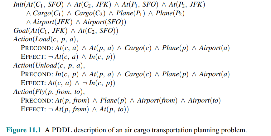
Example Domain: Air Cargo Transport

Air cargo transport problem involving loading and unloading cargo and flying it from place to place:

The following plan is a solution to the problem:

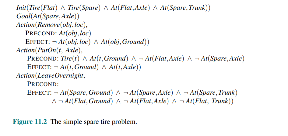
Example domain: the spire tire problem

Consider the problem of changing a flat tire. The goal is to have a good spare tire properly mounted onto the car’s axle.

The initial state has a flat tire on the axle and a good spare tire in the trunk.

To keep it simple, our version of the problem is an abstract one, with no sticky lug nuts or other complications. There are just four actions: removing the spare from the trunk, removing the flat tire from the axle, putting the spare on the axle, and leaving the car unattended overnight.

The solution is:

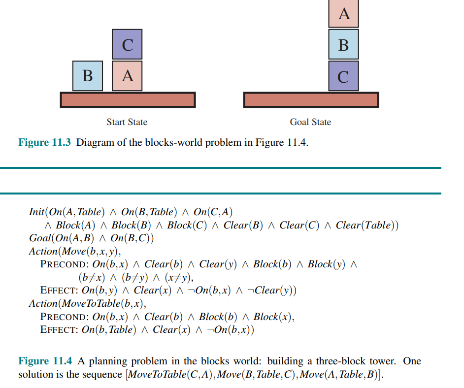
Example domain: the block world

One of the most famous planning domains is the blocks world. This domain consists of a set of cube-shaped blocks sitting on an arbitrarily-large table.

The blocks can be stacked, but only one block can fit directly on top of another. A robot arm can pick up a block and move it to another position, either on the table or on top of another block. The arm can pick up only one block at a time, so it cannot pick up a block that has another one on top of it.

A typical goal to get block A on B and block B on C:

We use to indicate that block b is on x, where x is either another block or the table. The action for moving block b from the top of x to the top of y will be .

One of the preconditions for moving is that no other block be on it. In FOL this would be , however basic PDDL does not allow quantifiers, so instead we introduce a predicate that is true when nothing is on .

The action Move moves a block b from x to y if both b and y are clear. After the move is made, b is still clear but y is not.
A first attempt at the Move schema is:

Misplaced &&\text{Action}(Move(b,x,y), \\ &\quad\text{PRECOND}:On(b,x) \wedge Clear(b) \wedge Clear(y), \\ &\quad\text{EFFECT}:On(b,y) \wedge Clear(x) \wedge \neg On(b,x) \wedge \neg Clear(y)) . \end{align*}$$ Unfortunately, this does not maintain Clear properly when x or y is the table. To fix this we do 2 things, first: $$\begin{align*} &\text{Action}(MoveToTable(b,x), \\ &\quad\text{PRECOND}:On(b,x) \wedge Clear(b), \\ &\quad\text{EFFECT}:On(b,Table) \wedge Clear(x) \wedge \neg On(b,x)) . \end{align*}$$ and second we take the interpretation of $Clear(x)$ to be "there is a clear space on $x$ to hold a block." Under this interpretation, Clear(Table) will always be true. ## Algorithms for classical planning The description of a planning problem provides an obvious way to search from the initial state through the space of states, looking for a goal. A nice advantage of the declarative representation of action schemas is that we can also search backward from the goal. We can have: - **Forward state-space search for planning**: - start at initial state - determine the applicable actions we unify the current state against the preconditions of each action schema - for each unification that successfully results in a substitution, we apply the substitution to the action schema to yield a ground action with no variables - **Backward search for planning**: - Start at the goal and apply the actions backward until we find a sequence of steps that reaches the initial state - Consider relevant actions at each step - Reduces branching factor - A relevant action is one with an effect that unifies with one of the goal literals, but with no effect that negates any part of the goal ![[../../../Attachments/Pasted image 20260604150424.png]] ### Forward state-space search for planning Planning problems can be solved by using heuristic search algorithms. [[AI - Lecture - Solving Problems by Searching - Heuristic Search Strategies and Heuristic Functions|heuristic search algorithms]]. The states in the search space are **ground states** where the fluents are either true or not. The **goal state** has all **positive fluents** in the problem's goal and none of the negative fluents. The **applicable actions** in state $s$, $Action(s)$ are grounded instantiations of the action schemas: - That is, constant values have replaced variables - They are **determined by unifying the current state against the preconditions** of each action schema - The **identified substitution** is applied to the **action schema** providing a **ground action with no variables** Each schema may unify in multiple ways: - If an action has **multiple literals** in the precondition, then each of them can potentially be **matched against the current state** in several ways - e.g. in spare tire, the Remove action, the precondition $At(obj, loc)$ matches against the initial state in two ways, resulting in the two subsitutions $\{obj/Flat, loc/Axle\}$ and $\{obj/Spare, loc/Trunk\}$. - This can lead to **search graphs** whose depth to the solution has an unfeasible number of nodes. An **accurate heuristics** is needed to make forward search **feasible**. >[!note]- How Forward state-space search for planning works > >1. Start from an initial state that is a **set of facts** i.e. `At(P1,SFO)` or `On(A, Table)`. >2. Look at all action schemas in your domain such as Fly, Load, Move, whatever. Look at the applicable ones i.e. the one where the precondition match with facts >3. This matching step is the unification: you bind variables in the action schema constants in the state. Once you find a valid binding, you get a concrete action instance >4. Once you have all applicable actions, each of them generates a successor state. You compute the next state by applying the action effects. Practically, this means you take the current set of fluents, remove the ones in the delete list, and add the ones in the add list. That gives you a new world state. >5. Somewhere in this expansion, you may reach a state that satisfies the goal condition. A goal state is simply one where all goal literals are true and the required negative are false. ### Backward search for planning Starts at the goal and works backward, applying actions to find a sequence of steps reaching the initial state. Focus on **relevant actions**, i.e., **with an effect that unifies with one of the goal literal**, but with no effect that negates any part of the goal. **Regression process**: given a goal $g$ and an action $a$, the regression from $g$ over $a$ yields a state $g'$ whose positive and negative literals are given by:

\begin{align} & POS(g′) = (POS(g) - ADD(a)) ∪ POS(Precond(a)) \ & NEG(g′) = (NEG(g) - DEL(a)) ∪ NEG(Precond(a)) \ \end{align}

g’ = In (C_2, p’) \land At(p’, SFO) \land Cargo (C_2) \land Plane(p’) \land Airport(SFO)

You can't use 'macro parameter character #' in math mode For most problem domains **backward search** keeps the **branching factor lower** than **forward search**. >[!note]- How backward search for planning works > >1. Start from the goal i.e. `At(Cargo1, SFO)` >2. Look for actions that could have been produced these goal conditions. An action is considered relevant if it has at least one effect that matches a goal literal. For instance, `Unload(Cargo1, P1, SFO)` is relevant because it produces `At(Cargo1, SFO)` >3. "Undo" logically that action by replacing the goal with what must have been true before that happens. This is the regression step. >4. The new regressed goal becomes a weaker requirement: it describes an earlier situation that would guarantee the original goal after executing the action. Repeat this process once you get to the initial state >5. Reverse the step lists to get a plan ### Other classical planning approaches **Planning Graph**: An approach called Graphplan uses a specialized data structure, a planning graph, to encode constraints on how actions are related to their preconditions and effects, and on which things are mutually exclusive. It is possible to encode a bounded planning problem (i.e., the problem of finding a plan of length k) as a [[AI - Lecture - Solving Problems by Searching - Constraint Satisfaction Problems|constraint satisfaction problem (CSP)]]. The encoding is similar to the encoding to a SAT problem, with one important simplification: at each time step we need only a single variable, $Action_t$, whose domain is the set of possible actions. An alternative called **partial-order planning** represents a plan as a **graph** rather than a linear sequence: - each **action** is a node in the graph - for each **precondition** of the action, there is an **edge** from another action (or from the initial state) that indicates that the predecessor action establishes the precondition. - So we could have a partial-order plan that says that actions Remove(Spare, Trunk) and Remove(Flat, Axle) must come before PutOn(Spare, Axle), without saying which of the two Remove actions should come first - We **search** in the space of plans rather than world-states, inserting actions to satisfy conditions ```mermaid graph TD Algorithms("Algorithms for classical planning") FW("Forward state-space search") BW("Backward search") Algorithms-->FW Algorithms-->BW FW-->FWStates("Ground States")-->InitialState("Initial State") FWStates-->FwGoalStates("Goal States") FW-->ApplicableActions-->FWUnification("Unification<br><small>matching</small>") FWUnification-->FWSubstitution("Substitution")--"Action Schema"-->FWGroundAction("Ground Action")--Execute-->FWSuccessorState("Successor State") BW--Start-->BWGoalStates("Goal State")-->BWRegression("Regression") BWRegression BWRegression-->BWSubgoal("Subgoal")--Repeat until-->BWInitialState("Initial State") ``` ## Heuristics for planning Recall from [[AI - Lecture - Solving Problems by Searching - Heuristic Search Strategies and Heuristic Functions|Heuristic Search Strategies & Heuristic Functions]] that an heuristic function $h(s)$ estimates the distance from a state $s$ to the goal, and that if we can derive an **admissible** heuristic for this distance, one that does not overestimate, then we can use $A^*$ search to find optimal solutions. An admissible heuristic can be derived by defining a **relaxed problem** that is easier to solve. The exact cost of a solution to this easier problem then becomes the heuristic for the original problem. Recall that a **search problem** is a graph where the nodes are states and the edges are actions. The problem is to find a path connecting the initial state to a goal state. There are **two main** ways we can **relax this problem** to make it easier: - by **adding more edges to the graph**, making it strictly easier to find a path - or by **grouping multiple nodes together**, forming an **abstraction of the state space** that has fewer states, and thus is easier to search. ### Heuristics that add edges to the graph The simplest is the **ignore preconditions heuristic**, which drops all preconditions from actions. Every action becomes applicable in every state, and any single goal fluent can be achieved in one step (if there are any applicable actions—if not, the problem is impossible). This **almost implies** that the number of steps required to solve the relaxed problem is the number of unsatisfied goals—almost but not quite, because: 1. (1) some action may achieve multiple goals and 2. (2) some actions may undo the effects of others. For many problems an accurate heuristic is obtained by considering (1) and ignoring (2). We can ignore only *selected* preconditions of actions. Consider the sliding puzzle (8-puzzle or 15-puzzle). We could encode this as planning problem involving tiles. We could encode this as a planning problem involving tiles with a single schema *Slide*:

\begin{align} & Action(Slide(t,s_1,s_2), \ & \quad PRECOND: On(t,s_1) \land Tile(t) \land Blank(s_2) \land Adjacent (s_1,s_2)\ & \quad EFFECT: On(t,s_2) \land Blank(s_1) \land \neg On(t,s_1) \land \neg Blank(s2))\ \end{align}

You can't use 'macro parameter character #' in math mode If we remove the preconditions $Blank(s_2) \land Adjacent(s_1,s_2)$ then any tile can move in one action to any space and we get the number-of-misplaced-tiles heuristic. If we remove only the $Blank(s_2)$ precondition then we get the Manhattan-distance heuristic. ![[../../../Attachments/Pasted image 20260604153721.png]] Another possibility is the **ignore-delete-lists heuristic**: removing the delete lists from all actions (i.e., removing all negative literals from effects). That makes it possible to make monotonic progress toward the goal. No action will ever undo the progress made by another action. It turns out it is still **NP-hard** to find the optimal solution to **this relaxed problem**, but an approximate solution can be found in polynomial time by [[AI - Lecture Solving Problems by Searching - Search in Complex Environments#hill-climbing-search|hill climbing]]. ### Domain-independent pruning Factored representations make it obvious that many states are just variants of other states. For example, suppose we have a dozen blocks on a table, and the goal is to have block A on top of a three-block tower. ![[../../../Attachments/Pasted image 20260604143110.png]] The first step in a solution is to place some block x on top of block y (where x, y, and A are all different). After that, place A on top of x and we’re done. There are 11 choices for x, and given x, 10 choices for y, and thus 110 states to consider. But all these states are symmetric: choosing one over another makes no difference, and thus a planner should only consider one of them. This is the process of **symmetry reduction**. With **symmetry reduction** we can prune out of consideration all symmetric branches of the search tree except for one. For many domains, this makes the difference between intractable and efficient solving. Another possibility is to do **forward pruning**, accepting the risk that we might prune away an optimal solution, in order to focus the search on promising branches. We can define a **preferred action** as follows: First, define a relaxed version of the problem, and solve it to get a **relaxed plan**. Then a preferred action is either a step of the relaxed plan, or it achieves some precondition of the relaxed plan. ### State abstraction in planning A **relaxed problem** leaves us with a **simplified planning problem** just to calculate the value of the heuristic function. Many planning problems have $10^{100}$ states or more, and relaxing the *actions* does nothing to reduce the number of states, which means that it may still be expensive to compute the heuristic. Therefore, we now look at relaxations that decrease the number of states by forming a **state abstraction**: a many-to-one mapping from states in the ground representation of the problem to the abstract representation. The easiest form of state abstraction is to ignore some fluents (relaxations that decrease the number of states). **Example**: - Consider the Air Cargo problem with 10 airports, 50 planes and 200 pieces of cargo. Each plane can be at one of 10 airports and each package can be either in one of the planes or unloaded at one of the airports. - So there are $10^{50} \times (50 +10)^{200} \approx 10^{405}$ states. - Now consider a particular problem in that domain in which it happens that all the packages are at just 5 of the airports, and all packages at a given airport have the same destination. - Then a useful abstraction of the problem is to drop all the $At$ fluents except for the ones involving one plane and one package at each of the 5 airports. Now there are only $10^5 \times (5 + 10)^5 \approx 10^{11}$ states. - A solution in this abstract state space will be shorter than a solution in the original space (and thus will be an admissible heuristic), - and the abstract solution is easy to extend to a solution to the original problem (by adding additional Load and Unload actions). A key idea in defining heuristics is **decomposition**: dividing a problem into parts, solving each independently, and then combining the parts. The **subgoal independence assumption** is that the cost of solving a conjunction of subgoals is approximated by the sum of the costs of solving each subgoal *independently*. The **subgoal independence assumption can be optimistic or pessimistic**: - optimistic when there are negative interactions between the subplans for each subgoal - pessimistic and therefore inadmissible when subplans contain redundant actions. Suppose the goal is a set of fluents G, which we divide into disjoint subsets $G_1, \dots , G_n$. We then find the optimal plans $P_1, \dots , P_n$ that solve the respective subgoals. What is an estimate of the cost of the plan for achieving all of G? We can think of each $COST(P_i)$ as a heuristic estimate, and we know that if we combine estimates by taking their maximum value, we always get an admissible heuristic. So $max_i Cost(P_i)$ is admissible, and sometimes it is exactly correct: it could be that $P_1$ serendipitously achieves all the $G_i$. ```mermaid graph TD Heuristics("Heuristics for planning") RelaxProblem("Relax Problem") Heuristics-->RelaxProblem RelaxProblem-->HAddEdges("Add Edges") HAddEdges-->IgnorePreconditionsHeuristic("Ignore Preconditions") HAddEdges-->IgnoreDeleteList("Ignore Delete-list") Heuristics-->DomainIndependentPruning("Domain Independent Pruning")-->ForwardPruning("Forward Pruning") DomainIndependentPruning-->SymmetryReduction("Symmetry Reduction") RelaxProblem--Relaxed Plan-->ForwardPruning Heuristics-->StateAbstraction("State Abstraction") StateAbstraction-->Decomposition StateAbstraction-->SubgoalIndAss("Subgoal Independence Assumption<br>{Positive, Negative}") ```