MML - Lecture 1 - Speech Recognition, LPC, Cepstra Coefficients, Dynamic Time Warping, Hidden Markov Models part 1

---

MML - Lecture 1

Speech Recognition

Speech Recognition deals with the problem of the recognition of the human speech. Grouped in two large families:

• speaker dependent
• speaker independent

Speaker dependent means that when the person that speaks changes, the performance go down. For example, Alexa can recognize words or short sentences spoken by people with different accents or languages, but performance may vary.

Another large difference is: speaking about connected and unconnected speech:

• Unconnected Speech: the speaker introduces pauses, even very shorts, between a word and another.
• Connected Speech: the speaker does not pause between words — speech flows continuously.

With unconnected speech, it’s generally easier for the system to segment and recognize individual words. On the other hand, with connected speech, it becomes harder to detect where one word ends and another begins, or to identify when a new utterance starts. Breaking the audio into individual phonemes or letters becomes much more challenging.

Currently, unconnected speech is where state-of-the-art models perform best. Most results are based on American English speakers. For example, on a dataset of spoken numbers by different speakers (without any speaker-specific tuning), the best recognition accuracy is around 95%.

A bit of historical context: MTMT

A bit of historical context: in the U.S., there used to be a massive telecom company called MTMT (similar to a national telecom provider). In the 1950s, telephone calls weren’t automated — if you wanted to call someone, you had to speak with a human operator who would manually connect you. The company wanted to reduce costs by replacing human operators with automatic speech recognition systems. That was one of the earliest motivations for developing speech recognition technology.

Speech Production

Speech Production Apparatus

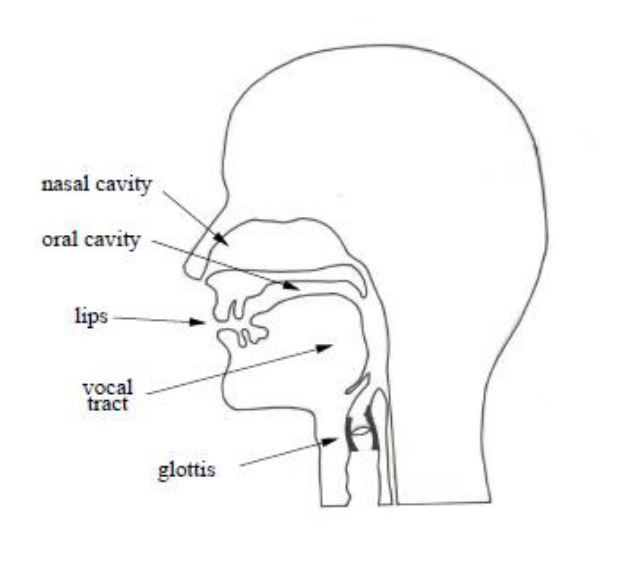The main components of the glottis are the vocal folds and the way they react with respect to air coming from the lungs enables to distinguish between the two main classes of sounds produced by human beings.

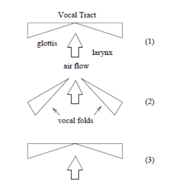The figure shows the glottal cycle:

1. the vocal folds open to requilibrate the pressure difference between larynx and vocal tract
2. Once the equilibrium is achieved the vocal folds close again
3. the cycle is repeated as long as air is pushed by the lungs

When the vocal folds vibrate, the sounds are called voiced, otherwise they are called unvoiced.

For a given language, all words can be considered like sequences of elementary sounds, called phonemes ,belonging to a finite set that contains, for western languages, 35-40 elements on average and each phoneme is either voiced or unvoiced.

Phoneme and Allophones

Phoneme: The phoneme is the Ideal sound unit with a complete set of articulatory gestures.

Allophones: is the set of all the variant of a given sound (“t” in eight against “t” in “top”).

Fundamental Frequency

When a voiced phoneme is produced, the vocal folds vibrate following the cycle described previously.

When air arrives at the glottis, the pressure difference w.r.t. the vocal tract increases until the vocal folds are forced to open to reestablish the equilibrium. When this is reached, the vocal folds close again and the cycle is repeated as long as voiced phonemes are produced.

The vibration frequency of the vocal folds is a characteristic specific of each individual and it is called the fundamental frequency F0. (timbro in italiano, timbr in english non è timbro).

The fundamental frequency is the single factor that contributes more than anything else to the voice pitch.

Formants

Most of the energy in human voices is distributed over the so-called formants, i.e., sound components with frequencies that are integer multiples of F0 and correspond to the resonances of the vocal tract.

Typical F0 values range between 60 and 300 Hz for adult men and small children (or adult women) respectively. This means that the first 10-12 formants, on which most of the speech energy is distributed, correspond to less than 4000Hz.

When we want to sample this signal (the voice), we need to sample it accoring to the Nyquist-Shannon theorem. That is 2x times the highest frequency present in the signal. So atleast 8000Hz.

Voiced and unvoiced phonemes

The production of unvoiced phonemes does not involve the vibration of the vocal folds. The consequence is that the frequency content of unvoiced phonemes is not as defined and stable as the one of voiced phonemes and that their energy is, on average, lower than that of the others.

Examples:

• voiced phonemes: milk or lag
• unvoiced phonemes can be found at the beginning of words six stop.

Articulators

The sounds produced at the glottis level must still pass through the vocal tract where several organs play as articulators (e.g., tongue, lips, velum). The position of such organs is defined articulators configuration and it changes the shape of the vocal tract. Depending on the shape, the energy is concentrated on certain frequencies rather than on others.

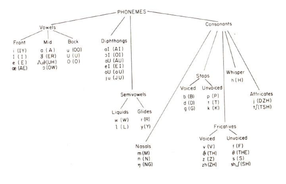
This makes it can reconstruct the articulator configuration at a certain moment by detecting the frequencies with the highest energy.

Since each phoneme is related to a specific articulator configuration, energy peak tracking, i.e., the detection of highest energy frequencies along a speech recording, enables, in principle, to reconstruct the voiced phoneme sequences and, since most speech phonemes are voiced, the corresponding words.

Speech Recognizer

Two modules:

• a speech feature extractor
• a classifier

Note

Here we have the classical machine learning approach, that needs a structured, lower-dimensional input. Therefore a speech feature extractor module is required. In deep learning we don’t have two modules because the speech feature extractor is embedded in the classifier. The feature extracture step is embedded in the learning of the neural network, like in the first layer for example, then the following layers act as classifiers to recognize phonemes and words.

Speech Feature Extractor

The old speech feature extractor were proposed in the 60s and 70s. The input is the digital electromagnetic signal, produced by the microphone, corresponding to the acustic signal emitted by the human speaker. It yields, as output, the features, extracted using single processing techniques. The features represent some spectral characteristic of the audio signal.

Linear Predictor Coding (LPC)

The idea behind Linear Predictor Coding (LPC) is the following. Given a speech sample, the sample s(n), at time n, can be represented as a function of a certain number of preceding samples. The peculiarity of the LPC is that the function is a linear combination (hence its name). Therefore we have,

In practice the audio signal is divided in frames (or window), each of 20ms. Then each frame is usually subdivided in 200 samples, sampling the signal at 0.1msec. (Empirically it works, there is no theory behind choosing these numbers).

LPC is an autoregressive process, that means that the current value of a signal is represented using previous values.

LPC is also quite similar to a time series. (backlink)

200 samples are used to estimate the (LPC coefficients) of the frame, using the least minimum square.

The coefficients can be represented in matricial form:

And the previous values of the series as:

The system is equivalent to the solution of matricial equation .

• where is the tensorial product, is the matrix of delays
• is the vector of LPC coefficients

Assuming that so the matrix is not singular. We can write:

• (square matrix)

Then we can write:

Since a popular choice is to fix , for each frame features are extracted by the LPC. LPC assumption: in the frame the signal has stationary dynamics.

Notice that, in practice there are other methods more efficients. The complexity of this algorithms scales as the cubic of , . Computing the inverse of a matrix is costly.

Cepstra Coefficients

It’s another way to extract the features, it works in a frame of 20ms the same framework as before.

The cepstrum of a digital signal is following:

Note this is similar to the inverse fourier transform, and so it means that transform the signals from frequency domain to temporal domain.

The word cepstrum

The word cepstrum has been obtained changing the order of syllables in the word spectrum. Cepstrum exists in a domain called quefrency (changing the syllables in frequency) that has temporal units.

In practice, the digital signal is divided in frames of 20 ms and for each frame cepstrum c(n) (usually for n=1…8) is computed. 8 cepstra coefficients are the extracted feature

LPC vs Cepstra

• Cepstra are more robust w.r.t noise and outliers
• LPC are faster to compute
• Starting from LPC it can compute cepstra coefficients

Time Warping

Classifiers in speech recognition must cope with the problem of comparing spectral sequences of different length.

We will also talk about Dynamic Programming similar to a particular type of dynamic programming: Longest Common Sequence.

Moreover, the comparison is harder since the same audio expression (utterance), emetted by the same speaker does not yield the same spectrum. Same utterance is not produced with the same speed (speaking rate). All these phenomena are called time warping.

Dynamic Time Warping

The first attempt was performed in 60s using dynamic programming. It was proposed the dynamic time warping.

In signal processing analysis, dynamic time warping (DTW) is one of the algorithms for measuring similarity between two temporal sequences, which may vary in speed. For instance, similarities in walking could be detected using DTW, even if one person was walking faster than the other, or if there were accelerations and decelerations during the course of an observation.

It’s a sort of generalization of the longest common sequence.

For example, in speech context, “hello” could be said slowly h---e---l---l---o or fast like hello. The key idea: it finds the minimum cumulative distance path between two sequences by stretching or compressing them in time.

In general, DTW is a method that calculates an optimal match between two given sequences with certain restriction and rules:

• Every index from the first sequence must be matched with one or more indices from the other sequence, and vice versa;
• The first index from the first sequence must be matched with the first index from the other sequence (but it does not have to be its only match).
• The last index from the first sequence must be matched with the last index from the other sequence (but it does not have to be its only match)

Also: The mapping of the indices from the first sequence to indices from the other sequence must be monotonically increasing, and vice versa. This means for example that if are indices in the first sequence, there must NOT exists two indices in the other sequence, such that the index is matched with index and index is matched with index and viceversa.

The optimal match is denoted by the match that satisfies all the restrictions and the rules and that has the minimal cost, where the cost is computed as the sum of absolute differences, for each matched pair of indices, between their values.

The sequences are “warped” non-linearly in the time dimension to determine a measure of their similarity independent of certain non-linear variations in the time dimension. This sequence alignment method is often used in time series classification.

Although DTW measures a distance-like quantity between two given sequences, it doesn’t guarantee the triangle inequality to hold.

In addition to similarity measure, a warped path is produced where the two signals are aligned in time.

• X(original) and Y(original) is transformed to X(warped) and Y(warped).

Note

This is similar to Needleman–Wunsch algorithm

Dynamic Time Warping Algorithm

• and are strings of discrete symbols but could also be for example the phoneme of human letters.
• is the distance between the symbols

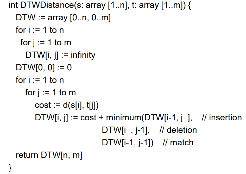
DTW implementation

To add a locality constraint we need to apply some changes. First the modification works only if 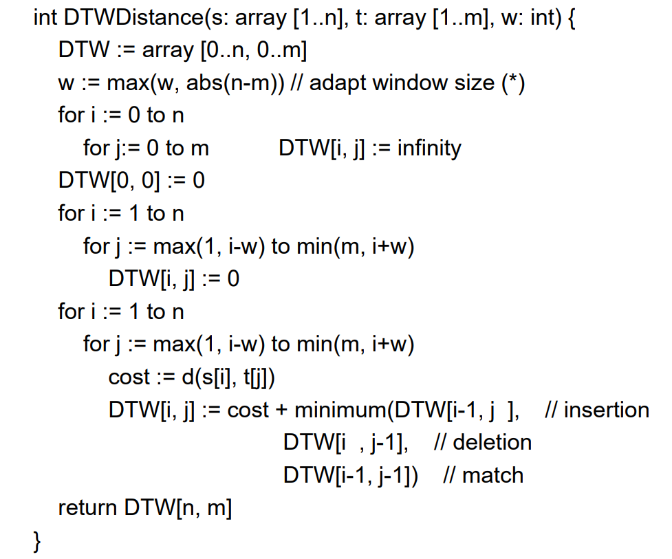, i.e the mid point is within the window length of the diagonal. So the window parameter must be adapted.

Dynamic Time Warping for Speech Recognition

It has been used until 80s. However, DTW is used in systems that, having moderate computational resources, can use only require simple speech recognizers.

DTW-based speech recognizers try to segment the spectrum in single phonemes that, then are classified using pattern recognition algorithms (e.g., K-Means).

The sequence of phonemes is compared, using DTW, with the words of the dictionary.

Hidden Markov Models

• See Markov Chain, Markov Models, Hidden Markov Models (HMM)

The standard technology used in the actual speech recognition systems. They do not segment the spectrum in the single phenomenes but try to recognize the word using the whole spectrum.

HMM musical example

We consider a music. It can be thought of as a sequence of notes: with different durations.

• the lower index is the starting note
• the high index is the last note

The single elements can be modeled as random variables, called state variables, which take values in a finite set: , i.e. for all , where . it’s the set of the of the notes, like .

Observation: means that the state variable at step takes value . For convention, altough not correct, we will say that the state at the step is .

Consider the case where the music score is at disposition and the sequence can be accessed directly. (note: music score is the “spartito”).

The probability of the sequence to be observed can be estimated through HMM of order , i.e. a probability distribution defined over sequences and based on the following conditional indipendence assumption:

i.e the state variable depends only on the state variables where . In other words it depends only on the previous state variables in .

This means that we do not consider . It’s a brilliant way to say that the memory of the system is of order .

As consequence the distribution can be decomposed as follows:

• means that it is , it does not depend on the productory.

In most cases, considering a MM of order is too cumbersone, so we consider , of order 1. This means that the probability depends only on the previous state. So the previous becomes:

That is completely specified by the initial state probabilities and by the transitional probabilities . This is not a restriction: any -th order MM can be represented with a first-order model by simply increasing the number of state variables.

MM and automaton

MM is a sort of probabilistic non deterministic automaton, therefore a generalization of the deterministic automaton.

Assumption: In principle, the transition probabilities depend on ; however, we focus on cases where they are homogeneous, i.e. they do not depend on t.

This assumption reduces significantly the number of parameters and enables one to collect all into a matrix , called transition matrix, such that

• where is the element of .
• first index is current state, second is previous state

Topology of the Markov Model

The transition matrix determines the topology of the MM, i.e the structure of the graph that can be used to represent an MM.

When transition between states and are not possible and not connection is established between their corresponding notes.

When then the state can be repeated in following steps along the sequence and the corresponding transition is called self-transition.

When only for or , the model is called Bakis. It means that can either stay in the same state or move to the next but never go backwards or skip.

From \ To	v₁	v₂	v₃	v₄
v₁	0.7	0.3	0	0
v₂	0	0.6	0.4	0
v₃	0	0	0.8	0.2
v₄	0	0	0	1.0
This is the visual transition possible:

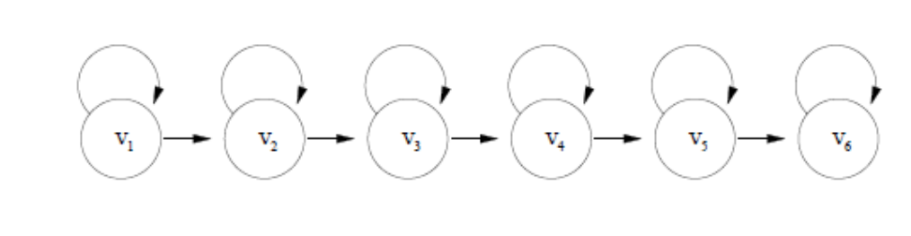When only for the model is called left-right. This structure is particularly suitable for data like speech where the sequence of states corresponds to a sequence of phonemes. With left-right model, you can’t go backwards but can skip ahead, like jump from straight to without passing for , as long as .

From \ To	v₁	v₂	v₃	v₄
v₁	0.5	0.3	0.2	0
v₂	0	0.4	0.4	0.2
v₃	0	0	0.7	0.3
v₄	0	0	0	1.0

The diagonal of the matrix is the part that identify that a state remains the same, so it’s a self connected state like previous picture.

When then the MM is said to be fully connected and each state can be followed by any other state.

From \ To	v₁	v₂	v₃	v₄
v₁	0.2	0.3	0.3	0.2
v₂	0.25	0.25	0.25	0.25
v₃	0.1	0.2	0.4	0.3
v₄	0.3	0.2	0.3	0.2

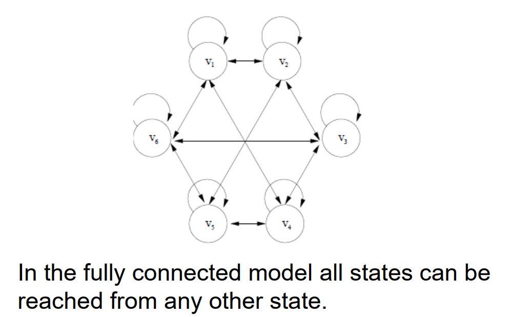
A model is said ergodic when any state can be reached by any other state in a finite number of steps.

From \ To	v₁	v₂	v₃	v₄
v₁	0.5	0.5	0	0
v₂	0	0.4	0.6	0
v₃	0	0	0.3	0.7
v₄	0.8	0	0.2	0

Means that you don’t need a direct transition, but you can always reach any state eventually through some path.

Hidden States

Consider now the case where the music score is not available and the only information at disposition about the music is a recording, i.e,. the sequence cannot be accessed directly and it is hidden.

The only possibility of modelling is to extract from the sound a vector of measures at each time step (for example using Cepstra Coefficients, but another possibility could also be to use a CNN).

Since measurement devices are not perfect and the players introduce variations even when they play the same note, the observations corresponding to a specific state are not constant, but rather follow a distribution .

As a consequence, the sequence hardly respects the Markov assumption, at least for small values.

Two assumptions: However, the observation sequence is the effect of the underlying state sequence which respects the Markov assumption, then it is possible to make the following simplifying assumptions:

i.e the probability of observation depends only on state and this last depends only on state .

With the second assumption we have deleted the contributions of the past observation. The state depends only on the previous state and not on the past observations. Itis a very strong assumption that simply the things a lot. In some other applications like bioinformatics it is not guaranteed that it works.

With the first assumptions, it depends only by the current state that depends on and not past states or past observations. Similar to [[../Computer Vision/CV - Theory - Tracking Linear Dynamical Models with Kalman Filters|[Computer Vision] Tracking Linear Dynamical Models with Kalman Filters]]

How a sequence of states is generated

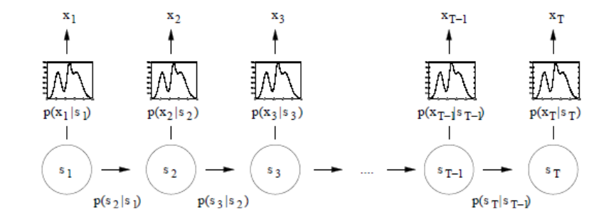The transition between the states is modeled by the transition probabilities , while the observations are generated following the emission probabilities .

Based on the previous independence assumptions, the joint distribution of observation and state sequences can be written as follows:

The joint distribution is completely specified by:

• A set of initial state probabilities → ;
• A transition matrix such that ;
• A set of emission probability functions → .

The set is called hidden Markov Model, because the states are not accessible directly, but only through the observations.

The Set can assume two different forms, either discrete or continuos.