SC - Lezione 15 - Minimization, Constrainted Minimization, Lagrange Multiplier, Least Square Variants

---

SC - Lezione 15

---

Checklist

Checklist

Domande, Keyword e Vocabulary

• Minimization
• derivative
• objective function
• gradient
• Matlab Gradient Function
• Properties of the Gradient
  • Perpendicular
  • 2-norm of the gradient
  • gradient and critical points
  • directional derivative
• Gradient computation in Matlab using Matlab’s Symbolic Toolbox
• symmetric matrix
• jacobian
• Constrainted Minimization
• Constraints
• machine example
• didactic example with constraint 2norm=1
• Lagrange Multiplier Technique
  • Solution of the constrainted minimization problem
• Recall of linear Least Squares problem and its variants
• Regularized LS
  • Penalty (Regularized LS)
  • Application of the penalty of regularized LS in AI
  • normal equation solution
  • SVD solution
• Weighted LS
• Lasso LS
  • 1-norm
  • sparse solutions
  • non-differentiability of the 1-norm
• Elastic Net LS
  • 2-norm and 1-norm

Appunti SC - Lezione 15

Minimization

• One of the main problem underlying AI

Formal definition

Let be a function (scalar function of several variables). The problem of minimization is denoted by:

we are interested more into the domain of , so the solution is a vector. More often you see also

The solution is called objective function. The solution of the problem is a point where assumes it minimum value

We don’t need algorithm for the maximum since we can compute and it’s the same.

2D gradient plot and approximate gradient calculation

Consider the function: recall that it has as many derivatives as his variable, that are assembled into a vector called the gradient.

Formally we can write that:

The gradient of a function of variables is the vector whose components are the partial derivatives of .

Matlab Gradient Function The gradient can be approximated on a grid using the matlab function gradient. It returns the one-dimensional numerical gradient of vector that representes the values of a 1D function on a 1D grid.

Properties of the Gradient

• If the gradient stays at a point where we plotted the contour line, the direction is always perpendicular to the contour line, passing for that point.

What do we expect at the center where the gradient is very small. When a derivative of a gradient is zero, it’s a critical point. The part of domain where the gradient is very small arrow then there is a maximum or minimum point here. The arrow goes into the direction of the maximum increase. On the left we have a minimum because it’s going outwards the arrow direction. on the right we have arrows that goes into, so it’s a maximum point.

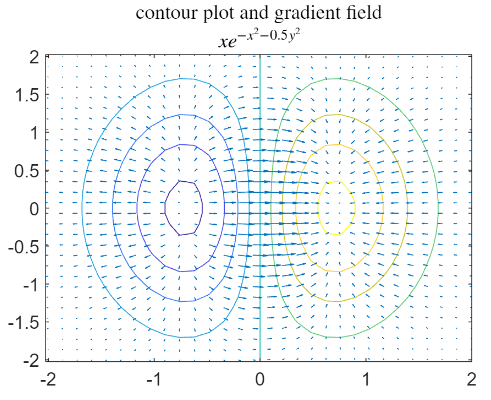
The derivative respect to x tell us this information: if it is positive and i goes into the x axis directions, it gives me the information about if the derivative is positive the function is decreasing. If i take a step outside the x-y axis, then i have the direction derivative.

Other properties to consider:

• The 2-norm of the gradient is proportional to the length of the arrow that represents it
• The gradient is zero at the critical points of the function
• The derivative in the direction (directional derivative) of a unit vector is given by the scalar product

Gradient computation in Matlab using Matlab’s Symbolic Toolbox

Gradients can also be computed exactly in symbolic form using the gradient command of the Matlab Symbolic Toolbox.

We consider the linear function where is a constant vector and is the vector of independent variables.

And we compute:

For example we have:

and

and we do

gradient(c'*x,x)

that tells us to compute the symbolci gradient of c'*x. That is

Now let’s consider another example with a symmetrix matrix . Recall that a symmetric matrix is a matrix where the elements above the diagonal are the same under the diagonal,

We compute , that is:

That is equal to

but since and because the matrix is symmetric, we have that:

Let’s consider now a vector function wich components functions:

(so we have 3 component functions) We compute the Jacobian matrix of the vector function that is:

Remind now that the rows of the Jacobian are the gradient of its component function, so we want to compute That is basically the same as doing:

Where we do the inner product of by the Jacobian matrix and the result is a vector:

It’s a generalization of the square of a function, of the example shown in the whiteboard.

If we consider the scalar function: and compute its gradient by y, and two times the jacobian matrix by y we obtain the same result.

Recall that:

(By the Chain Rule, recall from calculus how to compute the derivative of a composed function).

The result is 2 times the value of the function times the jacobian transposed.

So applying this property we get that:

Constrained Minimization

Consist in determining the minimum point of the objective function f in a subset (of its domain) formed by the points that satisfy predetermined conditions (constraints))

We want to compute the minimum of in this subset

where represents the constraints.

Machine example

We have a factory with three machines: ,, that produce two products and . occupies for 5 min, for 3 min, for 4 min. The production of one unit of occupies for 1 min, for 4 min and for 3 min. The net profit per unit of product is 30 Euros for and 20 Euros for . Which hourly production plan guarantees the maximum profit?

In this example we want to maximize the variable of profit. The Objective of the problem is: . The constraints are:

• The easier ones: and because you cannot produce -4 knifes, ofcourse.
• For in 1 hour (60 minutes), we have:
• For in 1 hour we have: :
• For :

We can solve in Matlab using the “linprog” function, which requires in input the vector of the coefficients that define the function to be minimized, the matrix and the vector of the linear inequality constraints, the matrix and the vector of the linear equality constraints, and the vector of the limiting constraints of the variables.

A = [5 1; 3 4; 4 3];   % matrix of linear inequalities
b = [60 60 60]';
x = linprog(-[30,20]',A,b,[],[],zeros(2,1)) % we don't have equality  constraints

Recall that any scalar function of variables can always be expressed as a scalar product of a constant vector and the vector representing the variables.

Didactic example with constraint 2-norm egual to 1

We have a nonlinear constraints: given a vector , we want to determine the vector with for which the scalar product assumes a maximum value:

Notice that is such that its 2 norm is equal to 1, we are not interested in any kind of x. It is well known a priori the result: the unit vector parallell to .

The solution find by matlab is the versor of the vector v: v/norm(v)

Or using the “fmincon” function that takes in input the function to be minimized, an initial approximation of the solution and the constraints.

Lagrange Multiplier Technique

(Backlink alla apposita lezione in ML) Is a mathematical tool that transforms a constrainted minimization problem subject to equality constraints:

into an equivalent unconstrainted problem, consisting in defining a new objective function called lagrangian defined as:

Where is called Lagrange Multiplier

Idea: If instead of considering a function of variables, since here the constraint is a scalar function, consider a function of variables. That is still a function of but also of another parameter called the lagrange multiplier.

Notice we just have plus the constraint function multiplied by a lagrange multiplier .

Generalizing this we have that: if is a vector function with constraints, we have that the Lagrangian becomes:

The solution to the systems of equations is: i.e finding the critical points by checking where the gradient is null. is the solution of the given constrainted minimization problem.

Suppose we want to solve the following problem:

and then impose that its gradient is equal to the null vector: .

In the following figure we show the previous constrainted minimum problem.

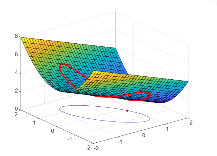The red point is the solution. As formulated above, we want the minimum only of the function restricted to the red circles.

Recall of linear Least Squares problem and its variants

We already saw the minimization problem of:

an we solved it in various ways, even in the full rank or not full rank variant (see SC - Lezione 11 - Applications of SVD in Least Square systems, Pseudoinverse matrix with SVD and Latent Semantic Analysis)

Sometimes in the applications this problem doesn’t appear like the classical ones.

Regularized LS - or Tikhonov or Ridge regularization

A common variant is called the regularized LS (also called Tikhonov or Ridge regularization).

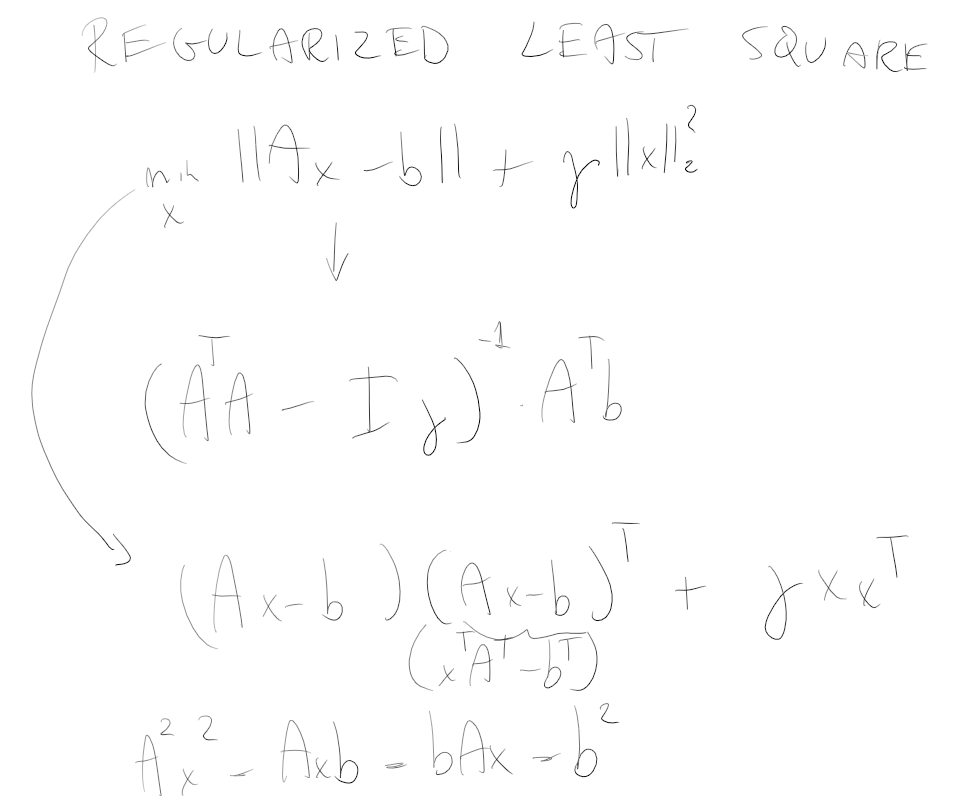
We want to minimize:

It’s the same but we added called penalty or regularized parameter

In AI this is sometimes used to avoid the overfitting. How? By favouring a solution with a small norm

Suppose that

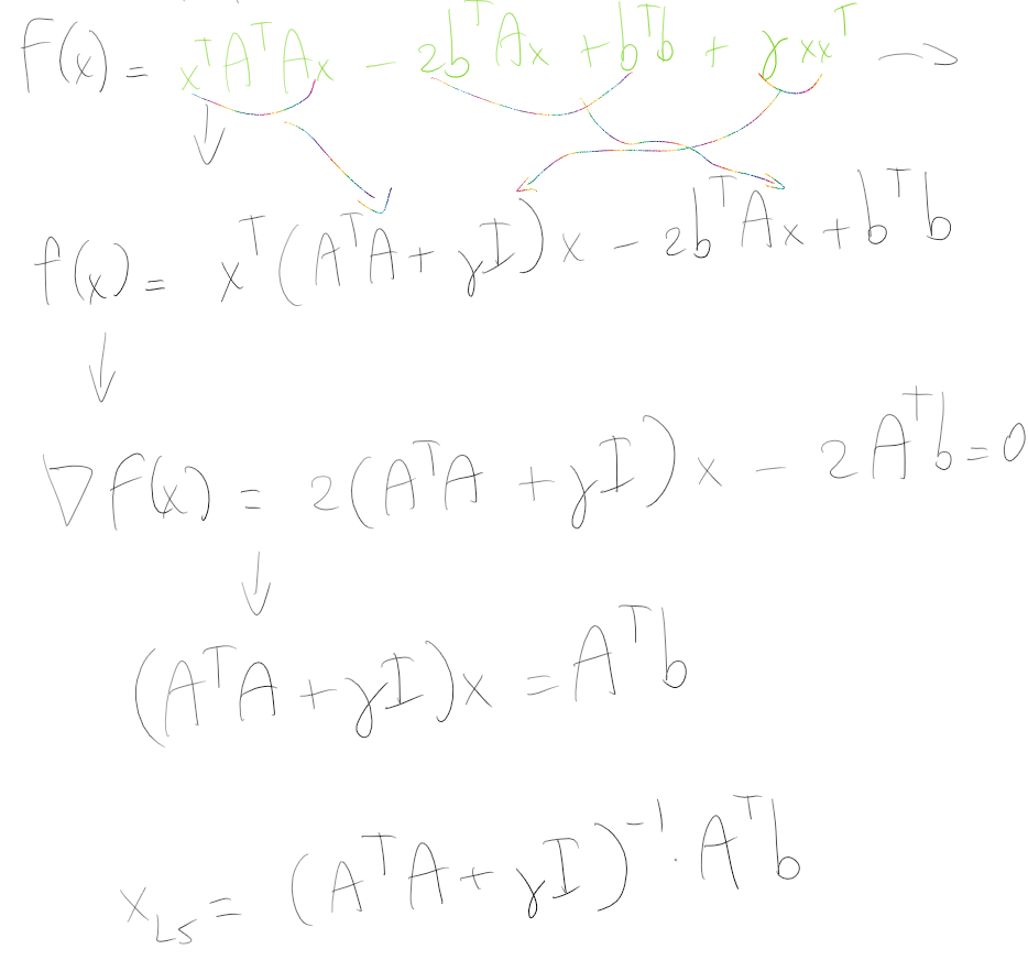
We can express the solution as in terms of normal equation as:

Passaggi dell’equazione normale

SVD x_LS solution

Or in term of SVD as:

Example.

Let’s consider the penalty parameter

We solve using our function and notice one thing: the norm of the residual of the standard LS problem is smaller, since its residual is orthogonal to the range of A, while the norm of the solution of regularized LS is smaller.

Weighted Least Square

Another common variant of Least Squares is Weighted Least Squares, where the matrix 𝐶 serves as a weight matrix that adjusts for the reliability of the data values in 𝑏.

whose solution can be expressed either in terms of normal equation:

And in terms of SVD:

Lasso Least Square

Another way of this kind of least square can appear is called Lasso (Least Absolute Shrinkage and Selection Operator)

It’s very similar to the regularized but the difference is that instead of 2-norm we have the 1-norm.

The aim of this problem is to favor solutions that are sparse.

For example, in digital photography, if you’re aiming to solve this problem while seeking a sparse solution (with a lot of zeros), this type of approach is necessary. The 1-norm here doesn’t have a direct analytical solutions since it is non-differentiable.

Elastic Net Least Square

Finally we consider the Elastic Net LS where both 2-norm and 1-norm are present:

The name suggests the flexibility of the solution that stretches (2-norm regularization) and compresses (1-norm regularization) to optimally fit the model to the data.

Both of the last two problems can be solved with lasso in Matlab.

---