Checklist
Domande, Keyword e Vocabulary
- Orthogonal projector
- Span
- QR factorization of a matrix
- Reduced QR factorization
- Trick to compute a reduced rank matrix
- Basis
- Orthogonal complement to the range of A
- Perpendicular vector
- QR Factorization for solving
- Expensiveness
- Normal Equations
- QR and Least Squares
- null space
- non decreasing function and analysis recall
- Pseudoinverse and the two ways to compute it
Appunti SC - Lezione 6
Orthogonal projector
The projection of
Multiplying
The result
Another way to see this is:
results in a square matrix called the Gram Matrix. It contains the dot products of the rows W with each other. - Then the gram matrix is multiplied by the vector x
QR factorization of a matrix
Any matrix A in
is an orthogonal matrix - R is a rectangular upper triangular matrix
.
Reduced QR Factorization
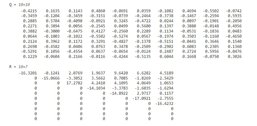 We can partition the matrix if we notice that
What happens if n < m and if m < n ?
Answer:
- if n < m, we are in the above case and we can do the Reduced QR factorization
- if m < n, the matrix R will not contains any NULL rows, so doing the Reduced QR doesn’t give me any advantage
This factorization qr() and adding 0 as argument of the function.
If we consider the matrix
Case of matrix with non Maximum Rank
I consider a matrix
Consider the code:
A = [A A*rand(5,2)]
[A A..]is append A and what on the right termA*rand(5,2)multiply a matrix A by a matrix
So we obtain a matrix that is linear combination of these two vectors.
Linear combination of the columns of A so the two last columns are a linear combination. They don’t contain new informations that isn’t contained in the first ones so the rank is reduced.
A random matrix is always a maximum rank matrix.
If i want a matrix 10 by 8 i need to compute a matrix that is a linear combination of the previous ones.
The matrix A*rand(5,2) that we append to A by doing [A A*rand(5,2)] it’s a matrix with only 2 columns because by doing
Now let’s consider 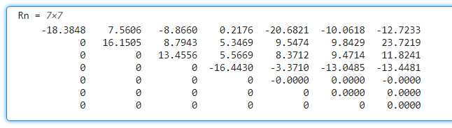 Notice how the last rows are null so it’s useless to multiply considering these two too.
If the matrix Qr = Q(:,1:r); Rr = R(1:r,:);
The remaining part of the matrix is Qmr = Q(:,r+1:m);
In math we write:
e
We observe that: norm(A-Qr*Rr,"inf")
Implications of the rank reduced QR factorization
The fact that the column of
Dimension reduction means that we want to find a lower-dimensional subspace of the original feature space and then project the data onto this subspace.
This process is aimed at retaining as much relevant information as possible while reducing the complexity and computational burden associated with high-dimensional data.
Clarification Example in data science terms
For example, in data science terms, if you have a 10-by-7 matrix, it means there are 7 features and 10 samples. If the matrix has a rank of 5, this tells us that the columns (which are 10-dimensional vectors) actually lie within a 5-dimensional subspace of this 10-dimensional space. Instead of considering all 10 dimensions, we are focusing on just 5 vectors that span this subspace. These original vectors can be represented by projecting them onto this lower-dimensional subspace, which is composed of only 5 basis vectors. This is the core idea behind dimensionality reduction.
The rank reveals that the data can be represented in a lower-dimensional subspace. You then find an orthogonal projection onto this subspace, and project the data into it, effectively reducing the dimensionality.
QR Factorization and Basis
After the QR factorization, any vector in the range of A can be represented in terms of the orthonormal basis given by the columns of Q. The matrix 𝑄 provides a new basis for the range of 𝐴, and these basis vectors are orthonormal (which is beneficial for numerical stability).
What about the remaining
This submatrix is a basis for the orthogonal complement of the range of A. The orthogonal complement to the range of A. You can easiliy use this submatrix to find an orthogonal component using this approach.
A vector
The null space of matrix
Exercise
Show that the columns of matrix V are orthogonal to the range of A
- Let A be a matrix, randomly generated Let V be the null space of A such that A^T V = 0
Solution:
V*V'*A(not this approach isn’t numerically stable but the values are almost near the zero)
QR factorization for solving Ax=b
We know that for solving
We can also solve
Multiply both sides on the left by
Since the matrix is square, this an upper triangular square system that can be solved by backward substitution.
We also showed in matlab that this method is more expensive for such a problem.
The QR can be used to solve particular sistems.
QR and Least Squares
They can be used for least squares systems, in particular when the rank is rectangular with
Recall that this kind of problem is defined as:
This problem doesn’t have a true solution, unless we find a vector
The solutions exists and it is unique of this problem.
We have that:
Recall the normal equation:
Theoretical justification for combining norm and square root.
If we have a function
From this principle, we derive:
represents the norm, represents the square function.
This framework provides a theoretical justification for why combining a norm with a square root (or square function) works mathematically.
Recall that when you multiply a vector by an orthogonal matrix, the size doesn’t change.
For this reason i can multiply both by
Now let’s consider the two vectors
by applying , becomes:
But
Let’s consider the term
where
This is just the sum of the two vectors so i splitted the sum, it is the minimum norm of these two vectors.
The second vector
and the solution
Pseudoinverse of a matrix with QR
The QR can be used to construct the pseudoinverse matrix
Suppose that we want to solve
Now, in this situation,
Since this is not a square matrix, i cannot write
Notice how i write
For finding the solution, i can use the QR factorization (see QR and Least Squares):
By this equation, we get the expression of the pseudoinverse of A
We also have another expression of the pinv: