Machine Learning Evaluation Metrics
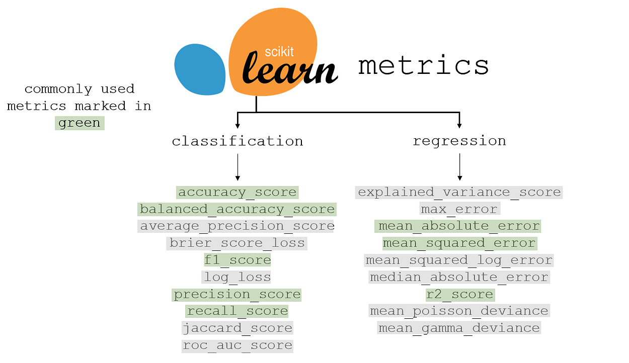
Regression metrics
Classification metrics
Classification Models have discrete output, so we need a metric that compares discrete classess in some form.
Classification Metrics evaluate a model’s performance and tell you how good or bad the classification is, but each of them evaluates it in a different way.
Accuracy
Is defined as the number of correct predictions divided by the total of number predictions
Top-K Accuracy
It is a generalization of accuracy score. The prediction is considered true as long as the true label is associated with one of the
is the indicator function
Precision
Precision is the ratio of true positives and total positived predicted.
TP = True Positive. FP = False Positive. See Confusion Matrix.
- If the precision is near to 1, then the model didn’t miss any true positives
- If the precision is toward 0, then the model has an high number of false positives which can be an outcome of imbalanced class or untuned model hyperparameters.
Recall
Is the ratio of true positives to all the positives in the ground truth.
TP = True Positive, FN = False Negative.
- Recall towards 1 means that the model didn’t miss any true positive
- Recall towards 0 means that the model has an high number of false negatives.
F1-Score
Uses a combination of Precision and Recall: in fact it is the harmonic mean of the two:
- An high F1 Score means that there is high precision and high recall
- A low f1 score means almost nothing: it doesn’t tell us if it’s low precision or low recall
F1-score macro, average and micro
The macro averaging (or macro-averaged F1 score) is the most straightforward one, it is computed using the arithmetic mean of all the per-class F1 Scores. This method treats all classes equally regardless of their support values.
Weighted averaging is computed by taking the mean of all the per-class F1 scores while considering each class’s support. Where support refers to the number of actual occurrences of the class in the dataset. The weight essentially refers to the proportion of each class’s support relative to the sum of all support values.
With weighted averaging, the output average would have accounted for the contribution of each class as weighted by the number of examples of that given class.
Micro averaging computes a global average F1 score by counting the sums of the True positive (TP), False Negatives (FN) and False Positive (FP). Micro-averaging essentially computes the proportion of correctly classified observations out of all observations. If we think about this, this definition is what we use to calculate overall accuracy.
When to use each one:
- for imbalanced dataset use macro average would be a good choice as it treats all classes equally
- for imbalanced dataset where you want to assign greater contribution to classes with more examples in the dataset, use weighted average1
Matthews Correlation Coefficient (MCC)
It measures the quality of binary (two-class) classifications. It is a correlation coefficient with values between
The statistic is also known as the phi coefficient.
Score Range:
Instead, when considering multiple class prediction, it can be defined as:
the number of times class truly occurred the num. of times class was predicted the num. of samples correctely predicted the total number of samples
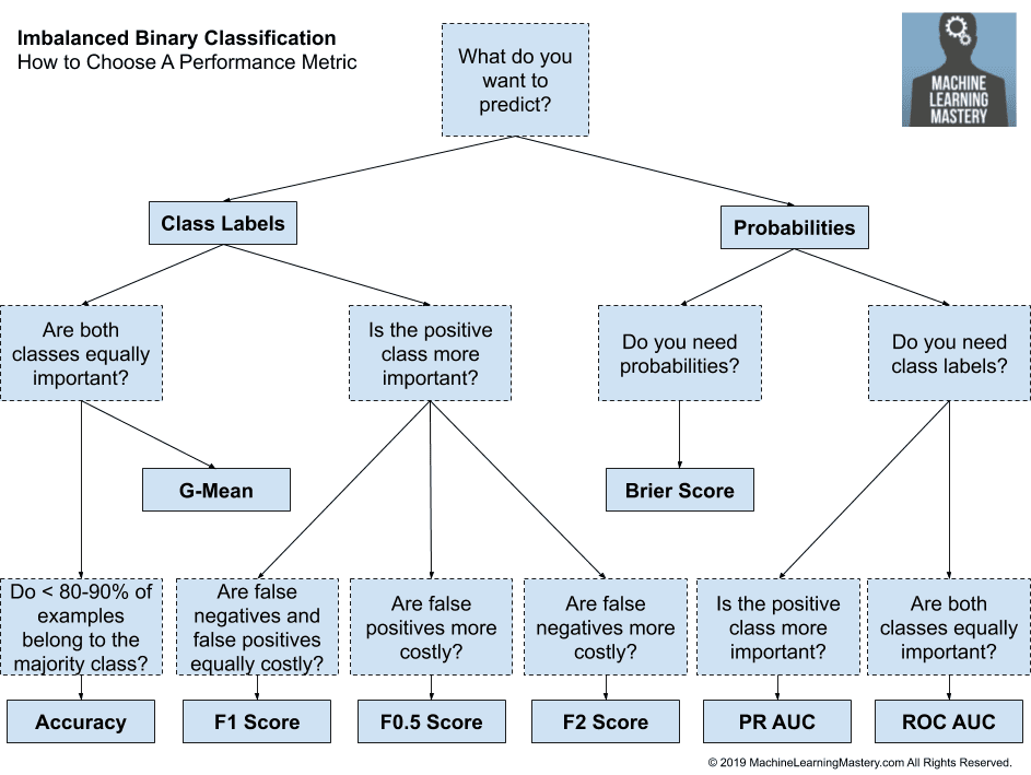
Metrics and Imbalanced Data
Standard metrics work well on most problems, which is why they are widely adopted. But all metrics make assumptions about the problem or about what is important in the problem. Therefore an evaluation metric must be chosen that best captures what you or your project stakeholders believe is important about the model or predictions, which makes choosing model evaluation metrics challenging.
Many of the standard metrics become unreliable or even misleading when classes are imbalanced, or severely imbalanced, such as 1:100 or 1:1000 ratio between a minority and majority class.
Sensitivity-Specificity Metrics for Imbalanced Data
Sensitivity
Sensitivity refers to the true positive rate and summarizes how well the positive class was predicted
Specificity
TN = True Negative. FP = False Positive.
G-Mean
Combining Sensitivity and Specificity we have G-Mean (Geomtric Mean)
Testing and Validating in Machine Learning
Usually your dataset is split into two sets: the training set and the test set. It is common to use 80% of the data for training and 20% of data for testing.
Holdout validation
Say that i have a linear model, but i want to perform some regularization, then i train 100 differente models with 100 different values for hyperparameter and find that the better converges at 5%. But when i launch this model into production, it does not perform well as expected and produces 15% errors. What just happened?
The problem is that i have measured the generalization error multiple time on the test set, so i have adapted the model and hyperparameters to produce the best model for that particular set.
A common solution to avoid this is called holdout validation: part of the training set is used to evalutate several candidate models and select the best one. The new heldout set is called validation set.
What you do now is to train multiple models with various hyperparameters on the reduced training set, then you select the model that performs best on the validation set. After this holdout validation process, you train the best model on the full training set, and this gives you the final model.
Recap:
- Split data into training set and test set
- Split test dataset into reduced test set and validation set
- Train different models with various hyperparameters on reduced test set and find the best model
- Train the best model with best hyperparameters on the full training set
This solution works well if the training set isn’t too small. Also, if the validation set is too large, then the remaining training set will be much smaller than the full training set.
To solve this problem you can use the cross-validation
Confusion Matrix
In the field of machine learning and specifically the problem of statistical classification, a confusion matrix, also known as error matrix, is a specific table layout that allows visualization of the performance of an algorithm, typically a supervised learning one; in unsupervised learning it is usually called a matching matrix.
For example, in a binary classification problem, where the value to predict is labeled as 0 or 1, a confusion matrix looks like this:
| Predicted 0 | Predicted 1 | |
|---|---|---|
| True 0 | 4000 | 122 |
| True 1 | 100 | 9000 |
In this case, the values Predicted 0 / True 0 mean that the model predicted correctly the data and matches the same datapoint from the test set. Predicted 1 / True 0 means that the model predicted 1 but the real value from the test set is 0
These outcomes are often called True Positive, False Positive, True Negative and False Negative