---

NLP - Lecture - MaskedLM §

• 10.pdf

Introduction to Masked LMs Language Models can treat text as casual (or left-to-right) relationship between words, see ([[NLP - Lecture - Transformers for NLP|[NLP] Introduction to Transformers]]). But what about tasks for which we want to peak at future tokens? Some important NLP tasks require understanding the entire sequence not just the past. Especially true for tasks where we map each input token to an output token. Examples:

• POS tagging i.e noun/verb labelling: we need future context because the correct tag may depend on later words
• NER tagging: i.e. identifying names, places, etc. : sometimes a later word clarifies the meaning.
• Sentiment Analysis i.e.

With masked language models, when computing the attention weight for a given token we not only consider the previous token and the current one but also the future tokens.

Bidirectional Transformer Encoders §

Decoder vs Encoder architecture We said that models of [[NLP - Lecture - Transformers for NLP|[NLP] Transformers]] are also called decoder-only because they correspond to the decoder part of the encoder-decoder model. By contrast masked language models are called encoder-only because they produce an encoding for each input token (that generally isn’t used to produce running text by decoding/sampling).

Bidirectional Transformer Encoders are used to compute very rich contextual representation for input token that can be used for other tasks. They are not used for generating text or predicting word but just to provide us with a rich contexutal representation for some sequence of tokens.

These encoders use masked self-attention, allowing each token to attend to all tokens in the sequence, both before and after:

• They take an input sequence of embedding vectors
• Produce a contextualized output embeddings:
• Each output vector contains information from the entire sequence (this implies every token is understood in its full context)

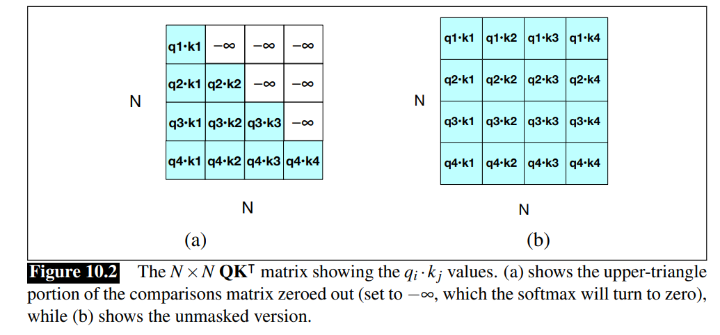
Recall that in Transformers for NLP - Parallelizing Attention we applied masks to avoid that the model access future tokens of the sentence. In this way the future is “blocked”.

In masked self-attention blocks, only some tokens are masked because the model must learn from both directions. This enables the model to learn deep contextual representations.

Architecture for bidirectional masked models §

Bidirectional transformer language models differ from casual transformers in two ways:

1. Attention is not casual: each token can attend to both previous and future tokens, not just the ones before it
2. Different training objective: instead of predicting only the next token at the end, they predict tokens in the middle of the text

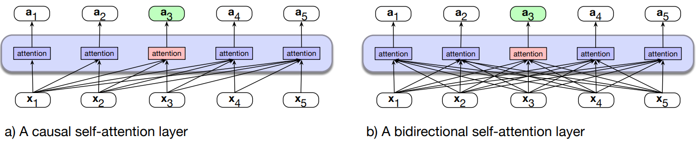
• (a) The casual transformer, highlighting the attention computation at token 3. The attention value at each token is computed using only information seen earlier in the context.
• (b) Information flow in a bidirectional attention model. In processing each token, the model attends to all inputs, both before and after the current one. So attention for token 3 can draw on information from following tokens.

Implementation: removing the mask - we simply remove the attention masking introduced in Transformers for NLP - Parallelizing Attention.

The single attention head equation becomes:

Like in casual transformers, the input is also a series of subword tokens, computed by one of the 3 popular tokenization algorithms. That means every input sentence first has to be tokenized, and all further processing takes place on subword tokens rather than words.

Example: original bidirectional transformer encoder model BERT The original english-only bidirectional transformer encoder model, BERT (Devlin et al, 2019) consisted of the following:

• English-only subword vocabulary consisting of 30,000 tokens generated using the WordPiece algorithm (Schuster and Nakajima, 2012)
• Input context window N=512 tokens, and model dimensionality d=768
• So X, the input to the model, is of shape .
• L=12 layers of transformer blocks, each with A=12 (bidirectional) multihead attention layers.
• The resulting model has about 100M parameters.

Example: XLM-RoBERTa: The larger multilingual XLM-RoBERTa model, trained on 100 languages has:

• multilingual subword vocabulary with 250,000 tokens generated using the SentencePiece Unigram LM algorithm (Kudo and Richardson, 2018)
• Input context window N=512 tokens, and model dimensionality d=1024, hence X, the input to the model, is of shape .
• layers of transformer blocks, with multihead attention layers each
• The resulting model has about 550M parameters.

Note that 550M parameters is relatively small as large language models go (Llama 3 has 405B parameters, so is 3 orders of magnitude bigger).

Training Bidirectional Encoders §

Cloze task: eliminating the causal mask in attention makes the guess-the-next-word language modeling task trivial, so a new training scheme is required. This is called cloze task, shown in the following example.

Casual LMs vs Masked LMs training example:

• For left-to-right LMs, the model tries to predict the last word from prior words:
  • The water of Walden Pond is so beautifully_____
• and we train to improve its predictions
• For bidirectional masked LMs, the model tries to predict one or more words from all the rest of the words:
  • The _________ of Walden Pond _______ so beautifully blue

The masked model generates a probability distribution over the vocabulary for each missing token. We use the cross-entropy loss from each of the model’s prediction to drive the learning process.

Masked Language Modeling (MLM) §

We consider this approach to training bidirectional encoders. MLM uses unannotated text from a large corpus.

In MLM training, 15% of the tokens are randomly chosen to be part of the masking. Example: “Lunch was delicious”, if delicious was randomly chosen, we have three possibilities:

• 80% token is replaced with special token:
  • Lunch was delicious Lunch was [MASK]
• 10% token is replaced with a random token (sampled from unigram prob):
  • Lunch was delicious Lunch was gasp
• 10% token is unchanged:
  • Lunch was delicious Lunch was delicious

We then train the model to guess the correct token for the manipulated tokens.

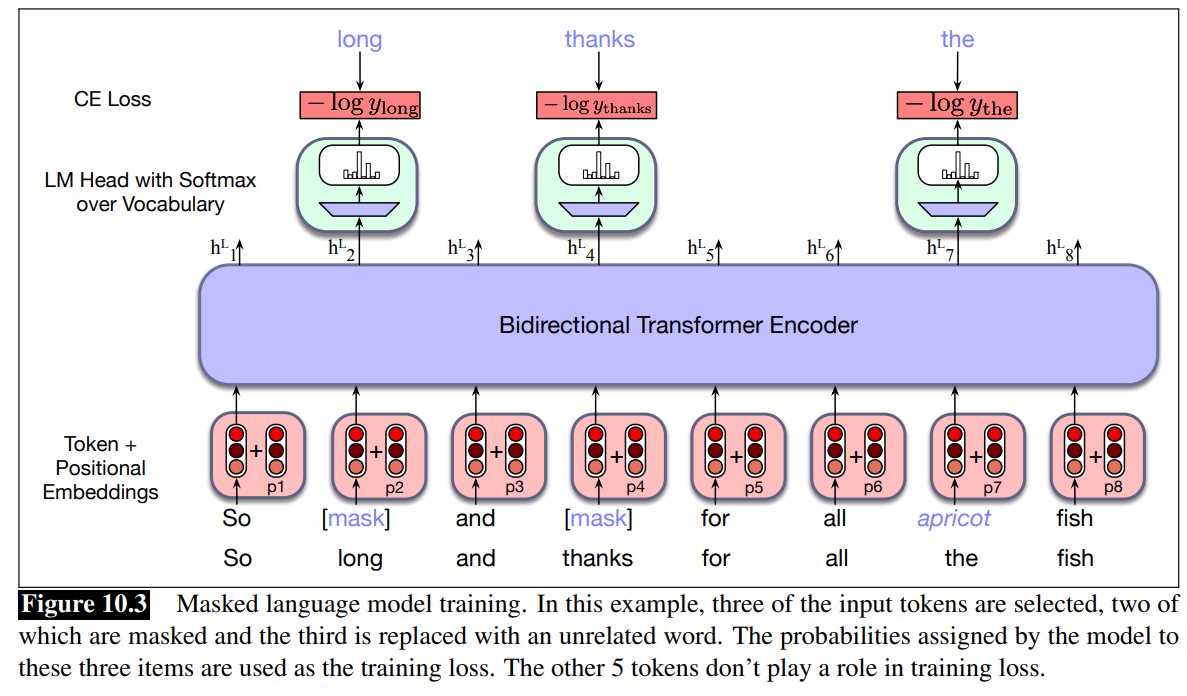
• First sentence is masked.
• Then token are added with positional embeddings
• Notice: when we compute the cross-entropy only for the mask tokens.

Now, let’s focus on just one token (since the parallelization and multi-head attention introduced in transformer - parallelizing attention, we know that these process happens simultaneously).

Recall from Transformer - Language Modelling head, that to produce a probability distribution over the vocabulary for each of the masked tokens, the language modelling head takes the output vector from the final transformer layer for each masked token , multiplies by an unembedding matrix to produce logits , and then uses softmax to turn the logits into probabilities over the vocabulary:

We can then use the cross-entropy loss (negative log probability) to compute the loss for each masked item.

Consider a given vector of input tokens in a sentence or batch . Let be the set of masked tokens. For a given input token corresponding for example to word “long”, the loss is the probability of the correct word “long”, given output :

We get the gradients by taking the average of this loss over the batch of sequences.

Note: only the tokens in (set of masked tokens) plays a role in learning; the other words play no role in the loss function. BERT and its descendents are inefficient since only 15% of the input samples in the training data are actually used for training weights.

Next Sentence Prediction (NSP) §

NSP is an auxiliary training task used in the original BERT model to help the model learn relationships between sentences.

While MLM teaches BERT how to understand words in context, NSP teaches BERT how sentences fit together.

Given two sentences, the model predict if they are a real pair of adjacent sentences from the training corpus or a pair of unrelated sentences.

BERT introduces two special tokens:

• [CLS] is preprended to the input sentence pair
• [SEP] is placed between the sentences, and also after the second sentence

And two more special tokens:

• [1st segment] and [2nd segment]
• These are added to the input embedding and positional embedding.

During the training, the output from the final layer [CLS] token is input to the classifier head (weights that predicts two classes:

Note that: some upgrade like RoBERTa do not use anymore this, because they demonstrated that this could be reached without this auxiliary task.

Next Sequence Prediction architecture:

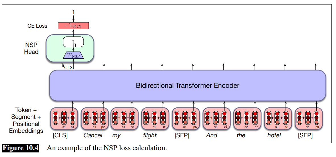
• The input is tokens to which segments and positional embeddings are added
• We are using a bidrectional attention model so we consider everything about the two sentences. This is enough to represent the relation between the two sentences.
• The head is a softmax layer, the output is then used to compute the CE loss.

Overwall, the loss function in BERT is composed of two terms:

• the first term related to the mask language model loss
• the second term is the cross entropy related to the next sentence prediction.

Training Regimes §

The original model was trained with 40 passes over the training data. Some models like RoBERTa drop NSP loss.

Tokenizer for multilingual models is trained from a stratified sample of languages (some data from each language).

Multilingual models are better than monolingual models with small number of languages. With a large number of languages, monolingual models in that language can be better. The “curse of multilinguality”: the performance on each language degrades compared to a model training on fewer languages.

For example the XLM-R model was trained on about 300 billion tokens in 100 languages, taken from the web via Common Crawl (commoncrawl.org).

Another problem with multilingual models is that they ‘have an accent’: grammatical structures in higher-resource languages (often English) bleed into lower-resource languages; the vast amount of English language in training makes the model’s representations for low-resource languages slightly more English-like (Papadimitriou et al., 2023).

Contextual Embeddings §

Given a pretrained language model and a novel input sentence, we can think of the sequence of model outputs as constituting contextual embeddings for each token in embeddings the input.

These contextual embeddings are vectors representing some aspect of the meaning of a token in context, and can be used for any task requiring the meaning of tokens or words.

More formally, given given the tokens , the model produces output vectors from its final layer .

The vector is typically used as the contextual embedding for token .

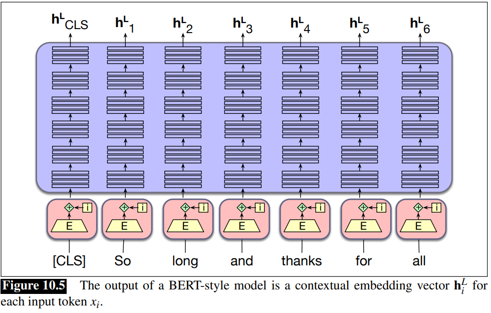
• Example: after the inference process, you get the vector of contextual embedding, one vector for each token.
• Consider the word and in the figure, and his contextual embedding .
• The same word and, in another context, would take a different vector representation, representing different meaning of the word in another sentence.

Instead of just using the vector from the final layer model, it’s common to compute the representation for by averaging the output from each of the last four layers of the model i.e:

Static vs Contextual Embeddings

• Static embeddings represent word types (dictionary entries).
• Contextual Embeddings represents word instances (one for each time the word occurs in any context/sentence)

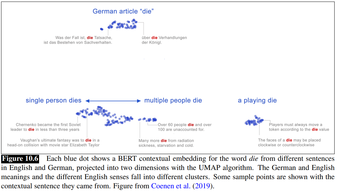
Word Sense Disambiguation §

Words are ambiguos as we know.

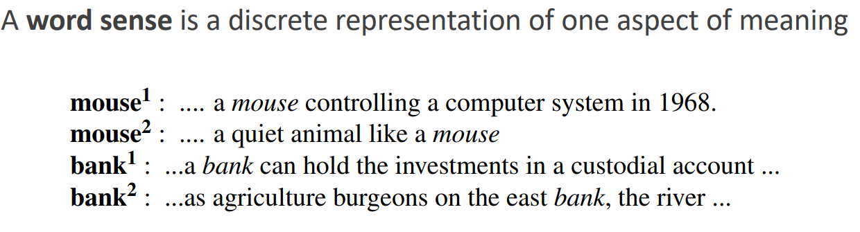
Contextual embeddings offer a continuous high-dimensional model of meaning that is more fine grained than discrete senses.

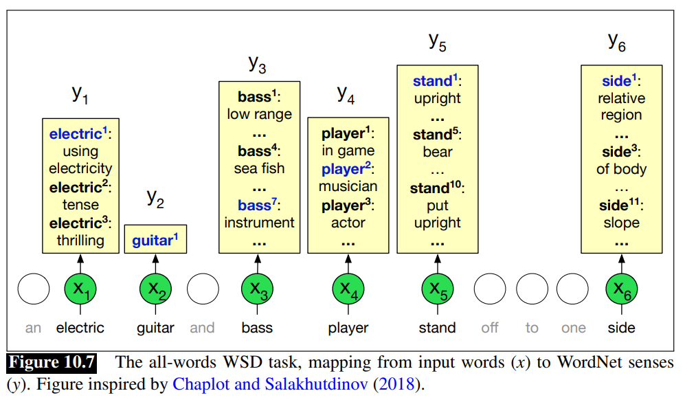
Word Sense Disambiguation (WSD) The task of selecting the correct sense for a word is called word sense disambiguation (WSD). WSD algorithms take as input a word in context and a fixed inventory of potential word senses (like the ones in WordNet) and output the correct word sense in context.

WSD can be a useful analytic tool for text analysis in the humanities and social sciences, and word senses can play a role in model interpretability for word representations.

Word senses also have interesting distributional properties. For example a word often is used in roughly the same sense through a discourse, an observation called the one sense per discourse rule.

1-Nearest Neighbour Algorithm for WSD The simplest and best performing WSD algorithm is the 1-nearest-neighbor algorithm using contextual word embeddings.

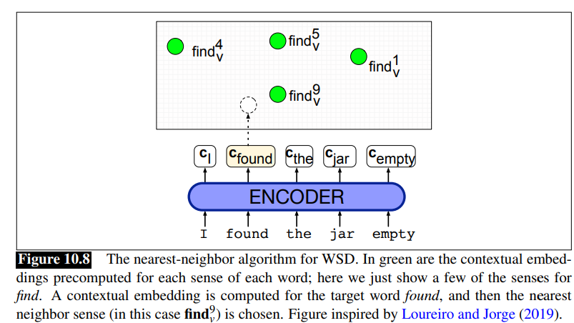
At training time we pass each sentence in some sense-labeled dataset (like the SemCore or SenseEval datasets in various languages) through any contextual embedding (e.g., BERT) resulting in a contextual embedding for each labeled token.

There are various ways to compute this contextual embedding for a token ; for BERT it is common to pool multiple layers by summing the vector representations of from the last four BERT layers.

Then for each sense of any word in the corpus, for each of the tokens of that sense, we average their contextual representations to produce a contextual sense embedding :

At test time, given a token of a target word in context, we compute its contextual embedding and choose its nearest neighbor sense from the training set, i.e., the sense whose sense embedding has the highest cosine with :

Word Similarity and Contextual embeddings §

We generally use cosine similarity like for static embeddings.

But there are some issues:

• Contextual embeddings tend to be anisotropic: al points in roughly the same direction, so have high inherent cosines (ethayarajh 2019). Note anisotropic is the contrary of isotropic
• One cause of anisotropy is that cosine measures are dominated by a small number of “rogue” dimensions with very high values (Timkey and van Schijndel 2021)
• Cosine tends to underestimate the human judgments on the similarity of word meaning for every frequent words (Zhou et al., 2022)

To allievate the issues, we can normalize (z-scoring) contextual embeddings: Given a set of of all the embeddings in some corpus, each with dimensionality (i.e., the mean vector and standard deviation in each dimension is:

Then each word vector is replaced by a standardized version :

However, human judgment underestimation still persists.

Fine-tuning for Classification §

Now that we have an architecture that captures contextual information for tokens, we can reuse it across many downstream tasks mentioned earlier.

Fine-tuning is a common way to do this. We take a pretrained language model and add a task-specific component, usually called a head, on top of it. The model’s output becomes the input to this head, which is trained using labeled data for the target task.

During fine-tuning, the pretrained model is usually kept frozen or only slightly updated, while the task-specific parameters are learned.

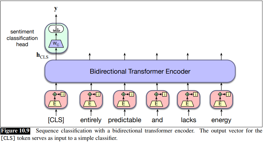
Sequence classification: the task of classify an entire sequence of text with a single label, like sentiment analysis or spam detection (see text classification). For sequence classification we represent the entire input to be classified by a single vector. For a pretrained BERT model, we add a new unique token to the vocabulary called [CLS] and propend it to the start of all input sequences, both during pretraining and encoding. The output vector in the final layer of the model for the [CLS] input represents the entire input sequence and serves as input to a classifier head, a logistic regression or neural network classifier that makes the relevant decision.

Finetuning a classifier for this application involves learning a set of weights, to map the output vector for the [CLS] token to a set of scores over the possible sentiment class. Assuming three-way sentiment classification task with classes (positive, negative, neutral).

To classify a document, we pass the input text through the pretrained language model to generate and multipltying it by and pass the resulting vector through a softmax:

Finetuning the values in requires supervised training data consisting of input sequences labeled with the appropriate sentiment class.

Sequence-Pair Classification §

Assign label to a pair of sequences. Some example of tasks:

• paraphrase detection (are the two sentences paraphrases of each other?)
• logical entailment (does sentence A logically entail sentence B?)
• discourse coherence (how coherent is sentence B as a follow-on to sentence A?)

We consider the same as special tokens as Next Sentence Prediction (NSP): we need both a [CLS] and [SEP] token.

To perform classification, the [CLS] vector is multiplied by a set of learned classification weights and passed through a softmax to generate label predictions, which are then used to update the weights.

Natural Language Inference (NLI) Consider the task of natural language inference (NLI) also called recognizing textual entailment.

For example in the MultiNLI corpus, pairs of sentences are given one of 3 labels: entails, contradicts and neutral.

These labels describe a relationships between the meaning of the first sentence (the premise) and the meaning of the second sentence (the hypothesis).

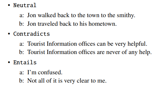
• A relationships of contradicts means that the premise contradicts the hypothesis
• entails means that the premite entails the hypothesis
• neutral means that neither is necessary true.

To finetune a classifier for the MultiNLI task, we pass the premise/hypothesis pairs through a bidirectional encoder as described above and use the output vector for the [CLS] token as the input to the classification head. As with ordinary sequence classification, this head provides the input to a three-way classifier that can be trained on the MultiNLI training corpus.

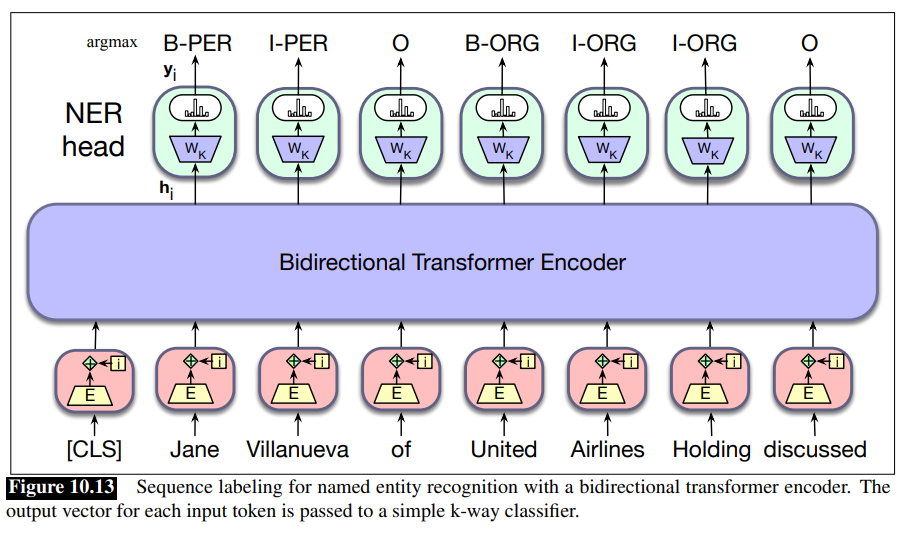
Fine-Tuning for Sequence Labelling: Named Entity Recognition §

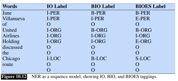
BIO Tagging §

We already introduced it in NLP - Named Entity Recognition. Entity Tags: Four entity tags are the most common: PER (person), LOC (location), ORG (organization) or GPE (geo-political entity).

BIO Tagging Since some entities could be composed of multiple words, BIO tagging and variantes (like IO, BIOES) are used. Recall BIO tagging a token is label with B if it starts a span of interest, I if it is inside a span of interest, O at the end of it.

The number of tags is for each token.

Sequence Labeling §

In sequence labeling, we pass the final output vector corresponding to each input token to a classifer that produces a softmax distribution over the possible set of tags.

For a single feedforward layer classifier, the set of weights to be learned is of size , where is the num. of possible tags for the task (assume BIO).

A greedy approach, where the argmax tag for each token is taken as likely answer, can be used to generate the final output sentence.

Let be a vector of probabilities over tags, and indexes the tags:

Tokenization and NER Note that the supervised training data for NER is typically in the form of BIO tags associated with text segmented at the word level.

For example in the following sentence containing two named entities: [LOC MT.Sanitas] is in [LOC Sunshine Canyon]

would have the following set of per-word BIO tags:

Mt   .  Sanitas is in Sunshine Canyon
B-LOC  I-LOC   O  O  B-LOC    I-LOC  O

Misalignement Problem The problem is the sequence of WordPiece tokens for this sentence doesn’t align directly with BIO tags in the annotiation. To deal with this misalignement, we need a way to assign BIO tags to subword tokens during training and a corresponding way to recover word-level tags from subwords during decoding.

• For training we can just assign the gold-standard tag associated with each word to all of the subword tokens derived from it
• For decoding, the simplest approach is to use the argmax BIO tag associated with the first subword token of a word. Thus, “Mt” would be assigned to “Mt.” and the tag assigned to “San” would be assigned to “Sanitas”, effectively ignoring the information in the tags assigned to ”.” and ""##itas”.

More complex approaches combine the distribution of tag probabilities across the subwords in an attempt to find an optimal word-level tag.

Evaluating Named Entity Recognition (NER) NER recognizers are evaluated by recall, precision and F1 measure:

• recall is the ratio of the number of correctly labeled responses to the total that should have been labeled;
• precision is the ratio of the number of correctly labeled responses to the total labeled;
• F1 measure is the harmonic mean of the two.

For NER, it is important not only to use a pretrained model, but also to update its weights. Studies show that relevant information flows from the middle layers to the final layers, so being able to fine-tune these layers can significantly improve performance. However, this is only effective if you have a very large labeled dataset, typically annotated with BIO tags.

When the dataset is smaller, it is safer to learn the task-specific weights () and fine-tune only a few layers of the pretrained model. Updating all layers in this case would likely cause overfitting and lead to poor generalization.

If you have very few training examples, the best strategy is to fine-tune only the classification head and keep the pretrained model completely frozen.

---