NLP - Lecture 16 - Part-of-Speech Tagging
- Prerequisite: NLP - Lecture 2,3 - Elements of Linguistics, in particular the syntax section.
Part-of-Speech (POS)
From the earliest linguistic traditions (Yaska and Panini 5th C. BCE, Aristotle 4th C. BCE), the idea that words can be classified into grammatical categories:
- part of speech, word classes, POS, POS tags
- 8 parts of speech attributed to Dionysius Thrax of Alexandria (c. 1st C. BCE):
- noun, verb, pronoun, preposition, adverb, conjunction, participle, article.
See syntactic analysis for common abbreviations.
These categories are relevant for NLP today.
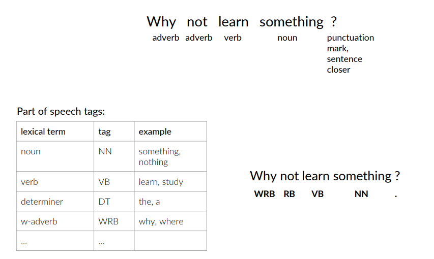
POS Tagset
Part-of-speech (POS) tags are lexical categories such as noun, verb adjective, pronoun, preposition, article, etc. They are also known as word classes or morphological classes.
We call a tagset the set of all POS tags used by some model. Different languages, different grammatical theories, and different applications may require different tagsets.
POS is a clue to sentence structure and meaning.
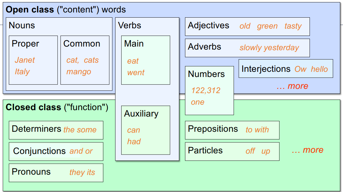
Opened vs Closed words
POS tags fall into two broad categories: closed class and open class
Closed-class words usually include function words: short, frequent words with grammatical function:
- determiners: a, an, the
- pronouns: she, he, I
- prepositions: on, under, over, near, by, …
They are relatively fixed membership: new words in this class are rarely coined.
Open-class words usually consist of content words: nouns (including proper nouns), verbs, adjectives, and adverbs:
- Plus interjections: oh, ouch, uh-huh, yes, hello
- New words appear almost always in this class
- E.g., iPhone (noun), to fax (verb)
The Universal Dependencies (UD) tagset
The UD tagset contains 17 tags
- POS tagged corpora for 92 languages

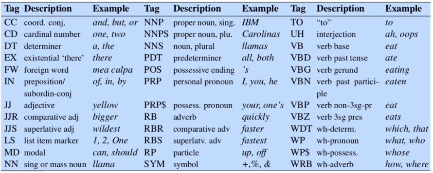
The English-specific Penn Treebank tagset
The English-specific Penn Treebank (PTB) tagset is also very popular
- it contains 45 tags
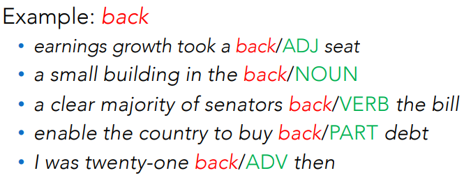
Example: Tagged English Sentences
- Using UD tagset
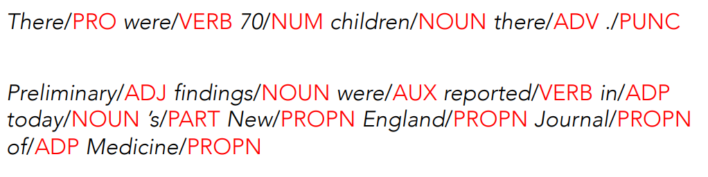 Notice that the same word can have different tags in different sentences or within the same sentence.
We need also to make decisions about segmentation, for instance punctuation or the English ‘s is often segmented off as a particular
Part-of-speech tagging
Definition: assigning a proper (unique) part-of-speech tag to each word in a sentence.
POS tagging must be done in the context of an entire sentence, based on the grammatical relationship of a word with its neighboring words.
It is an instance of a more general task called sequence labeling
Tagging is a disambiguation task: words are ambiguous, depending on the context in which they appear, they may have different tags.
Example: The word ‘book’ can be tagged as VERB or as a NOUN:
- Book/VERB that flight
- Hand me that book/NOUN
The goal is to find the correct tag for the situation.
The input sequence
We assume that the tagset is fixed, not part of the input:
Structured prediction task:
In POS tagging we need to output a whole sequence of tags
The number of output structures can be exponentially large in the length of the input, which makes structured prediction more challenging than classification.
Why POS Tagging?
Can be useful for other NLP tasks:
- Parsing: POS tagging can improve syntactic parsing
- MT: reordering of adjectives and nouns (say from Spanish to English)
- Sentiment or affective tasks: may want to distinguish adjectives or other POS
- Text-to-speech (how do we pronounce “lead” or “object”?)
Or linguistic or language-analytic computational tasks
- Need to control for POS when studying linguistic change like the creation of new words, or meaning shift.
- Or control for POS in measuring meaning similarity or difference.
How difficult is POS tagging?
Roughly 15% of word types are ambiguos, hence 85% of word types are unambiguous. For instance, Janet is always PROPN, hesitantly is always ADV.
But those 15% tend to be very common, so ~60% of word tokens are ambiguous.
POS Evaluation
The accuracy of a POS tagger is the percentage of test set tags that match human gold labels.
Human ceiling: how often do human annotators agree on the same tag? For PTB this is around 97%. Accuracies over 97% have been reported across several languages, using the UD tagset.
POS Tagging Performance in English
How many tags are correct? (Tag accuracy)
- About 97%
- Hasn’t changed in the last 10+ years
- HMMs, CRFs, BERT perform similarly
- Human accuracy about the same
Most frequent class baseline: is the stupidest possible method and has a performance of
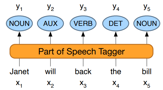
Sources of information for POS tagging
Janet     will     back     the     bill
      AUX/NOUN/VERB?             NOUN/VERB?
Part of speech taggers generally make use of three sources of information:
- Prior probabilities of a word having the tag: “will” is usually an AUX
- Identity of neighboring words: from english language rules, ”the” is a determinant, the next word is usually a noun. So an automatic target can exploit this knowledge to assign noun and not i.e verb.
- Morphology and wordshape:
- Prefixes: unable, “un” is for ADJ
- Suffixes: importantly, “-ly” is for ADJ
- Capitalization: Janet: first letter capital is for nouns
Standard methods for POS tagging
Supervised Machine Learning Algorithms:
- Hidden Markov Models
- Alternatives to HMM: Conditional Random Fields (CRF) / Maximum Entropy Markov Models (MEMM)
- Neural sequence models (RNNs or Transformers)
- Finetuning Large Language Models (like BERT), finetuned
All these require a hand-labeled training set, all about equal performance (97% on English):
- All make use of information sources we discussed
- Via human-created features: HMMs and CRFs
- Via representation learning: Neural LMs
Markov chains
The Hidden Markov Model (HMM) is based on augmenting the Markov chain model.
A Markov chain is a model that expresses the probabilities of sequences of random variables, the states, taking values from some set. Words, tags, or symbols representing anything, e.g., the weather.
A Markov chain assumes that if we want to predict the future in the sequence, all that matters is the current state.
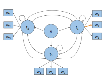
How it’s used in POS tagging:
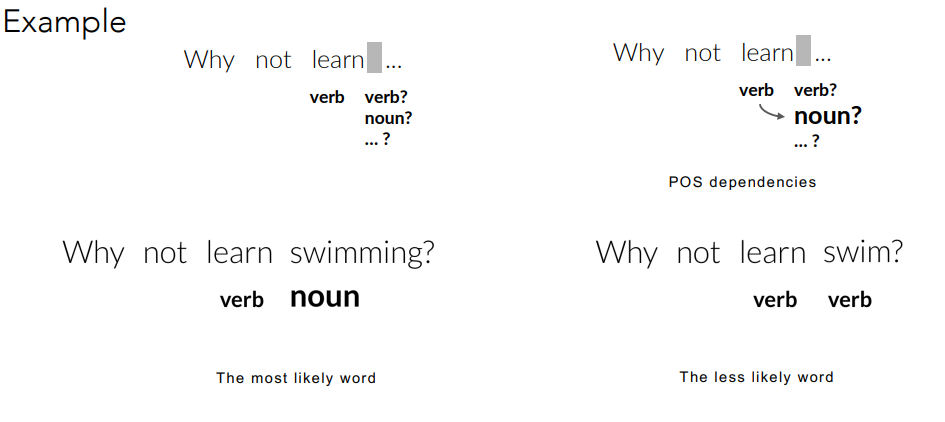
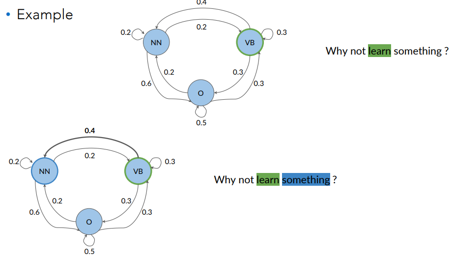
The idea is that the likelihood of the next word’s POS tag in a sentence tends to depend on the POS tag of the previous word.
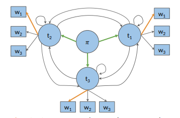
We can visually represent the likelihoods of the next word pos tags in the following figure:
A Markov chain is a stochastic model that describes a sequence of possible events. To get the probability for each event, it needs only the states of the previous event. It can be depicted as a directed graph.
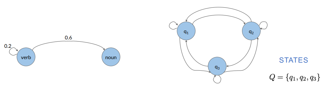
POS tags as states & transition probabilities
The parts of speech tags are events that can occur.
To go from one state to another state we define a term that we call transition probabilities. Transition probabilities express the chances of going from one POS tag to another.
They are the arrows in the following figure:
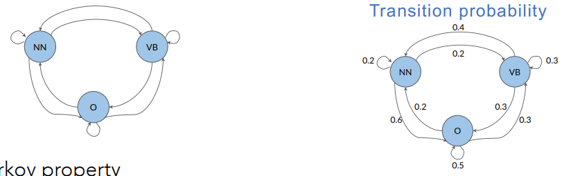
Markov Property: the probability of the next event only depends on the current event. All one needs to determine the next state is the current state.
Transition Matrix
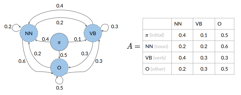
States and transition probabilities are stored in a table (transition matrix), equivalent but more compact representation of the Markov chain model.
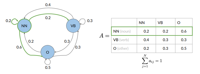
A transition matrix is an
On row we have tags, and on the column the same tag. Being in the noun tag, what is the probability of going to another noun (0.2), of going to adverb (0.2) and to getting the O (other tag) it’s 0.6. Considering the second row, we can do the same with verb.
Since transition matrix entries represents probabilities, the sum of all the row’s entries should be 1:
How about the first word of the sentence? We introduce an initial state.
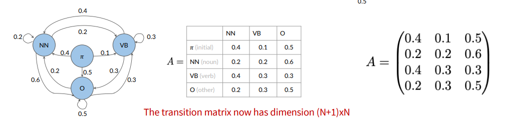
In general, given a set of states 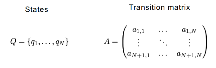 The initial probabilities are in the first row.
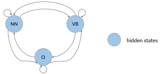
We don’t know what are the probabilities of going from a tag to another tag, so we need to infer the corresponding part of speech. This tag is represented in Hidden Markov Models as hidden states. POS tags are the hidden states. We only observe words.
Hidden Markov Model (HMM)
An HMM is a probabilistic sequence model.
Given a sequence of units (words, letters, morphemes, sentences, whatever), it computes a probability distribution over possible sequences of labels and chooses the best label sequence (with Viterbi algorithm).
An HMM allows talking about observed events (like words we see in the input) and hidden events (like POS tags) that we think of as causal factors in our probabilistic model.
HMM vs MM: Markov Model uses transition probabilities to go from one POS tag to another. But these states are hidden because they are not directly observable from the text data. Rather, the words within a phrase are observable (what the machine sees).
Hidden Markov Models make use of emission probabilities that give us the probability to go from one (hidden) state (POS tag) to a specific word:
Transition probabilities in HMM
The transition probabilities are represented by an
Emission probabilities in HMM
They describe the transition from the hidden states of a HMM, which are parts of speech, to the observables or the words of a corpus
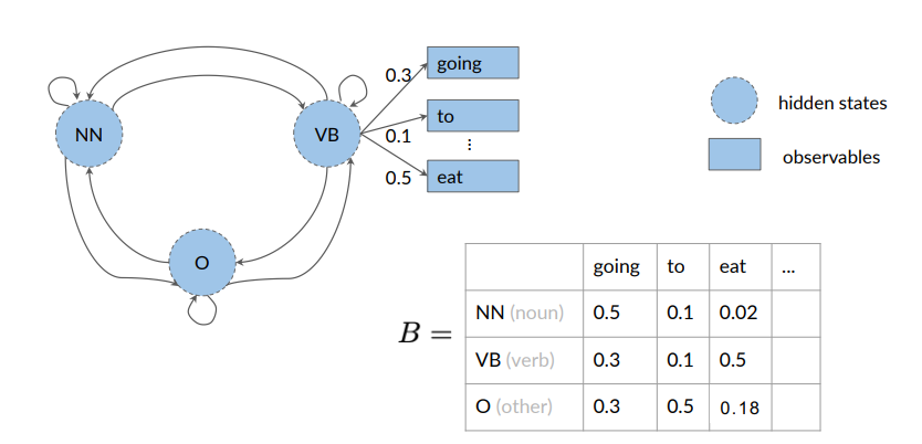
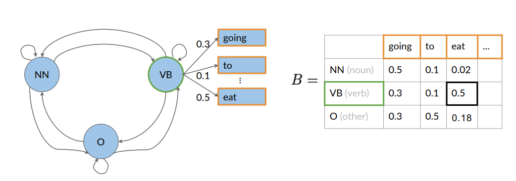
The row sum of probabilities is one:
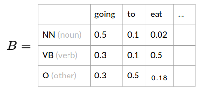
In this example, there are emission probabilities greater than zero for all three of our parts of speech tags. This is because words can have different parts of speech tag assigned depending on the context in which they appear.
For example:
- “He lay on his back”, back is a noun
- “I’ll be back”, back is an adv.
Transition and Emission matrices
Given a set of states
We have a transition matrix:
And an emission matrix
Where:
=number of states =number of words
Calculating Probabilities for transition and emission matrices
Given a corpus, let’s see how to compute the probabilities for the transition and emission matrices.
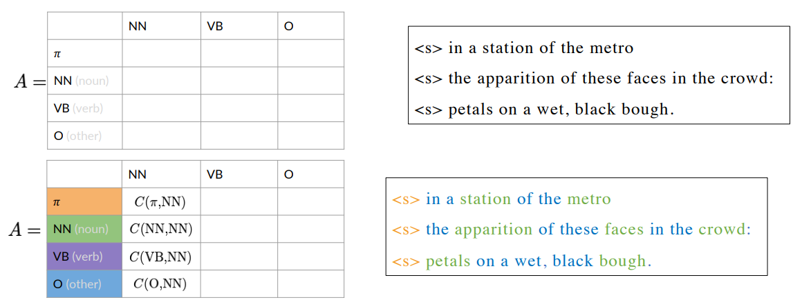
To calculate the transition probabilities, we only use the parts of speech tags from the training corpus.
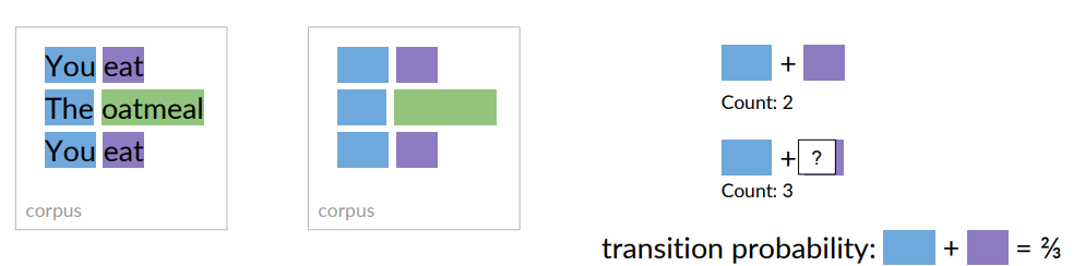
Example: To calculate the probability of the blue parts of the speech tag, transitioning to the purple one, counts the occurrences of that tag combination in the corpus, which is two
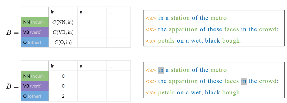
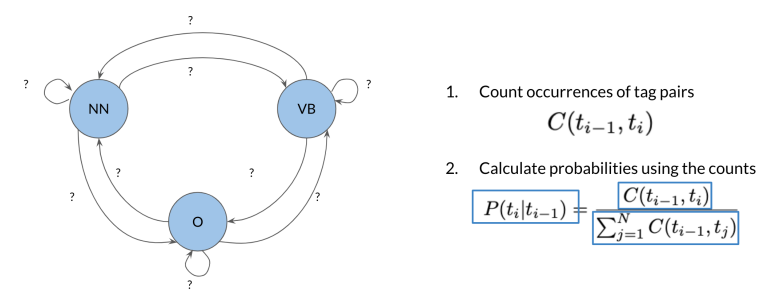 More formally, to calculate all the transition probabilities of the Markov model, we’d first have to count all occurrences of tag pairs in the training corpus:
- is the count of times that tag (i-1) shows up before tag i.
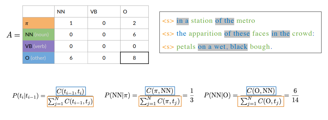
Then, we can calculate probabilities using the counts. In particular, we can compute the probability that a tag shows up after another tag:
- At the numerator we have the count of the occurencies that tag
shows up before tag - At the denominator we have the sum of the counts that tag
shows up before all the others tag .
Example
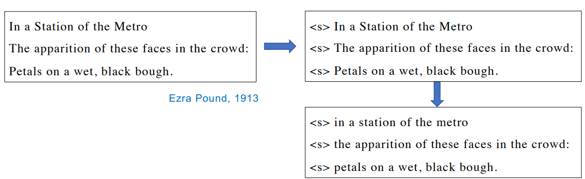
Let’s consider a little example corpus (Haiku, shorts Japanese poetry). Before any tagging activity, preprocess it by adding a starting symbol for each sentence and lowering all the letters.
To populate the transition matrix, you need to calculate the probability of a tagging
happening, given that another tag already happened.
Smoothing
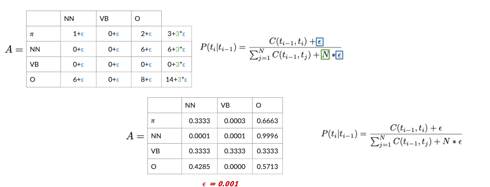
In the previous example we have two problems:
- The row sum of the (verb) VB tag is
, which would lead to a division by 0. - Lots of entries in the transition matrix are 0, meaning that these transitions will have a probability of 0
This won’t work if you want the model to generalize to other Haiku, which might contain verbs.
One simple solution is to add to every entry in the table
We count the co-occurrences of a POS tag with a specific word. Example:
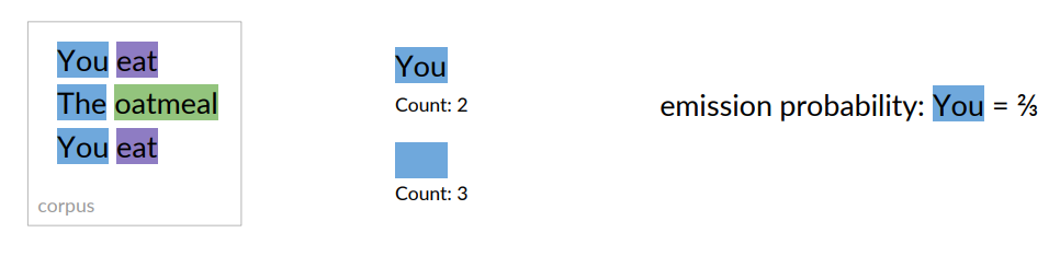 Count how often a word is tagged with a specific tag (e.g., NN, VB or O):
If
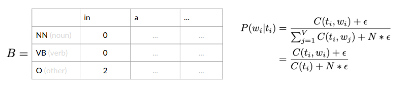
Smoothing leads to a better generalization.
HMM POS tagging as decoding
The task of finding the sequence of hidden states that best explains a sequence of observations is called decoding.
In POS tagging, the observations are words from the vocabulary, and the hidden variables are the POS tags. Given an input sequence of words, decoding means finding the corresponding sequence of tags.
Formally, in an HMM we are given:
- transition matrix
- emission matrix
- A sequence of observations
Goal: find the most probable sequence of states
For POS tagging, this means choosing the tag sequence
Since we talk about “most probable”, we can use the Bayesian Theory of Decision.
Using Bayes rule, the problem becomes computing:
We can drop the denominator
HMM assumptions: HMM taggers make two further simplying assumptions.
First, the probability of a word appearing depends only on its own tag (is independent of neighboring words):
Second, the probability of the next tag depends only on the previous tag (rather than the entire tag sequence):
Plugging these assumptions into
The two parts of last equation correspond to the
The decoding algorithm for HMMs is Viterbi Algorithm.
Same assumptions and problem is described also in [[../Multimodal Machine Learning/MML - Lecture 1 - Speech Recognition, LPC, Cepstra Coefficients, Dynamic Time Warping, Hidden Markov Models part 1#Hidden Markov Models|[MML] - HMM for Speech Recognition]].
The Viterbi Algorithm
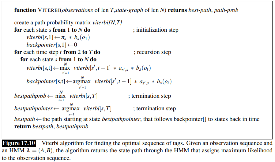
Viterbi algorithm is an instance of dynamic programming, so it resembles the minimum edit distance.
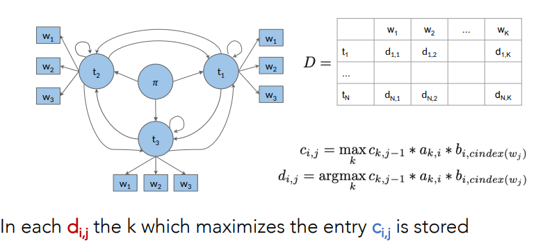
The Viterbi algorithm first sets up a probability matrix or lattice, with one column for each observation
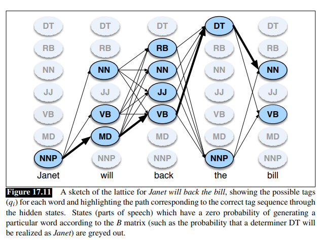
Consider this figure, using as example the sentence Janet will back the bill
Each cell of the lattice,
The value of each cell is computed by recursively taking the most probable path that could lead us to this cell.
Like other dynamic programming algorithms, Viterbi fills each cell recursively.
For a given state
The three factors that are multiplied in this equation for extending the previous paths to compute the Viterbi probability at time
: Previous Viterbi path probability from previous time step. : transition probability value (from transition matrix) from previous state to current state : the state observation likelihood of the observation symbol given the current state .
Viterbi Algorithm: working Through an example
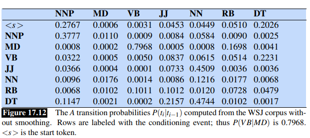
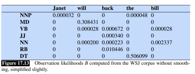
Consider the following two tables:
Goal: We want to tag correctly the sentence Janet will back the bill into: Janet/NNP will/MD back/VB the/DT bill/NN.
The word Janet only appears as NNP, back has 4 possible parts of speech, the word the can appear as determiner or as an NNP (in titles like “Somewhere Over the Rainbow”, all words are tagged as NNP).
- There are N=5 state columns
- Column 1 is for word janet, col 2 for will, col 3 for back, col 4 for the and col 5 for bill as you can a see at the bottom
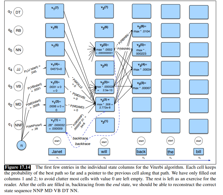
- We start with
<s>and so the probability that the first word is i.e a NNP given start symbol. - Notice that most of the cells in the first column are zero since the word Janet cannot be any of those tags.
- Next each cell in the will column gets update.
- For each state we compute the value
viterbi[s,t]by taking the maximum over the extensions of all the paths from the previous column that lead to the current cell according to equation(seen before) - Each cell gets the max of the 7 values from the previous column, multiplied by the appropriate transition probability; as it happens in this case, most of them are zero from the previous column.
- The remaining value is multiplied by the relevant observation probability and the (trivial) max is taken
- If you fill the lattice and backtrace, it should return the gold state sequence NNP MD VB DT NN
Viterbi Algorithm (taken from slides)
Decoding objective: finding the most probable sequence of tags. Involves breaking down the joint probability
Goal: maximize the probability of the tag sequence
Why emission matrix:
- words in a sentence naturally influence each others: HMM captures this indirectly via tag transitions
- conditionally independent: we assume
, and once we know the tag (e.g., NN), the word choice is treated as independent of neighbours - Computational cost: without this assumption, we would need to calculate dependencies across the entire sequence that is computationally impossible
- Trade-off: while words are not truly independent in NL, treating them as conditionally independent given their tags allows us to break the problem into small, multiply-ble parts.
Viterbi Algorithm: Steps
- Initialization
- Forward pass
- Backward pass
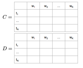
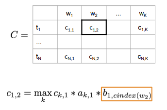
Auxiliary matrices
holds the intermediate optimal probabilities holds the indices of the visited states - size
, = number of POS tags, = number of words in the given sequence.
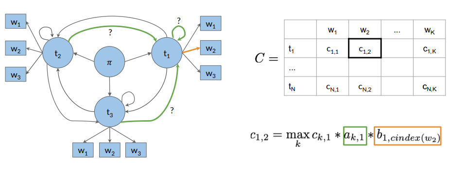
First, columns of matrices
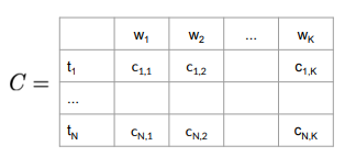
Initialization Step for C Matrix
For matrix
returns the column index in the emission matrix for given word .
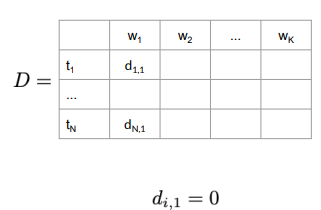
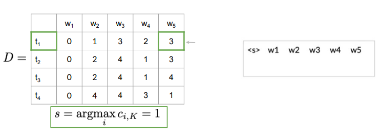
Initialization Step for D Matrix:
The first column has all entries 0 as there are no preceding POS tags traversed.
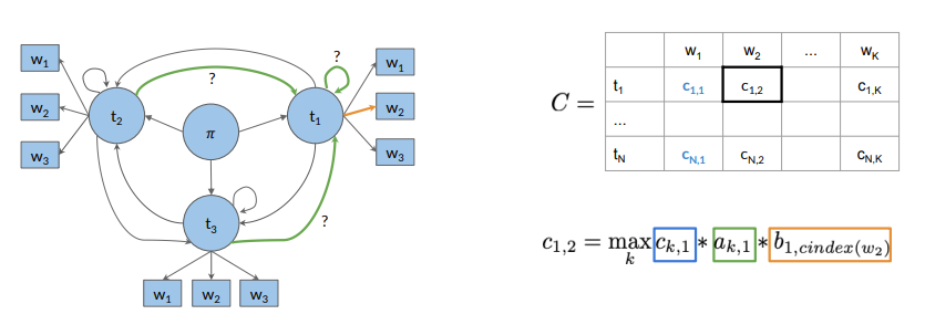
Forward Pass
For example:
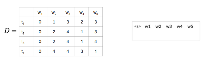
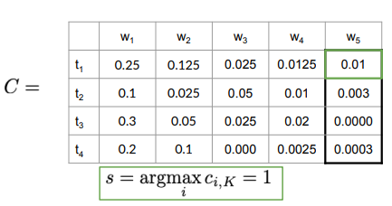
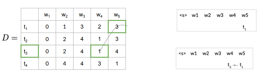
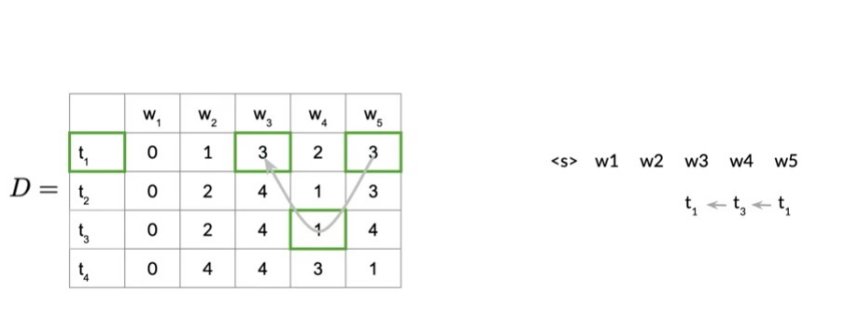
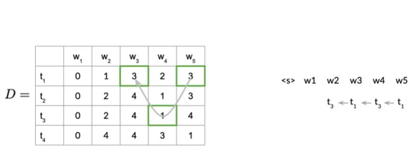
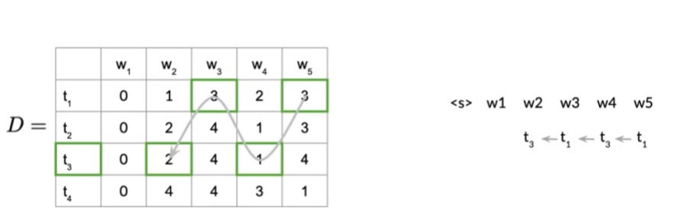
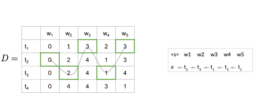
Backward Pass
After the forward pass, we have the matrices
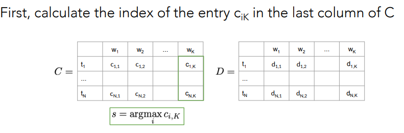 Example:
Named Entity Recognition
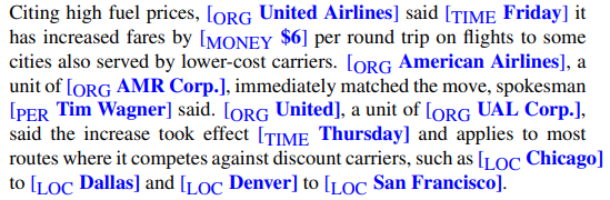
A named entity is, roughly speaking, anything that can be referred to with a proper name: a person, a location, an organization.
The task of named entity recognition (NER) is to find spans of text that constitute proper names and tag the type of named entity recognition NER the entity.
Four entity tags are most common: PER (person), LOC (location), ORG (organization), or GPE (geo-political entity).
Why NER:
- Useful first step in lots of natural language processing tasks.
- In sentiment analysis we might want to know a consumer’s sentiment toward a particular entity
- Entities are a useful first stage in question answering, or for linking text to information in structured knowledge sources like Wikipedia.
- Central to tasks involving building semantic representations, like extracting events and the relationship between participants
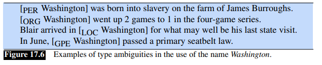
NER challenges POS tagging, unlike NER, does NOT have segmentation problem, since each word gets one tag.
NER is harder because the ambiguity of segmentation make the task harder since we need to decide what’s an entity and what isn’t, and where the boundaries are.
Another difficulty is caused by type ambiguity:
BIO Tagging
How can we turn this structured problem into a sequence problem like POS tagging, with one label per word?

We label any token that begins a span of interest with the label B, tokens that occur inside a span are tagged with an I and any tokens outside of any span of interest al labeled with O.
We’ll have distinct B and I tags for each named entity, and only one O tag.
The number of tags is thus
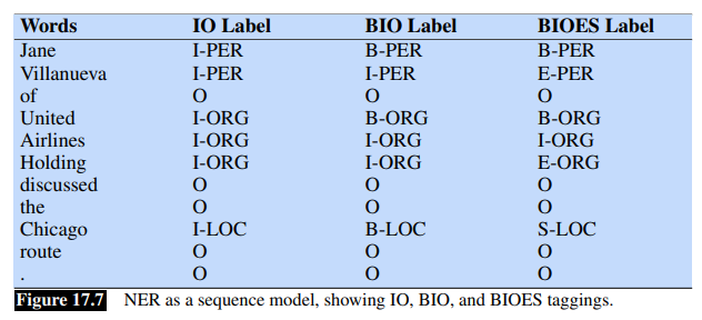
The example shows also the variants IO tagging (no B tag), and BIOES tagging with adds an end tag for the end of a span and a span tag S for a span consisting of only one word.
A sequence labeler (like HMM, but also RNN, Transformer etc) is trained to label each token in a text with tags that indicate the presence (or absence) of particular kinds of named entities.
Evaluation of Named Entity Recognition
Instead of using accuracy, NER is evaluated with recall, precision and
This is justified by the fact that for a named entity tagging, the entity rather than the word is the unit of response. For example, two entities “Jane Villanueav” and “United Airlines Holding” and the non-entity would count as single response.
Also, a system that labeled Jane but not Jane Villanueava as a person would cause two errors, a false positive for O and a false negative for I-PER.
In addition, having entities as unit of response lead to a mismatch between the training and the test conditions.
As alternative to HMM for POS tagging, see also Conditional Random Fields (CRF)