NLP - Lecture - Sequence Models, RNN, LSTM, Encoer-Decoder in NLP

---

NLP - Lecture - Sequence Models §

• 13.pdf

Modeling Time in Neural Networks §

Language is inherently temporal. Yet the simple NLP classifiers we’ve seen (for example sentiment analysis) mostly ignore time.

Motivations §

N-Gram based language models scale poorly with the sequence length.

A better scaling can be achieved by using parametrized models based on neural networks.

However:

1. NN has a fixed number of inputs and outputs wheres we need to handle different lenght sequences in the training and test sets
2. If a word or group of words in a given location in the sequence represents a concept, then the same word (or group of words) at a different location is likely to describe the same concept that the new location.

A Recurrent Neural Network has a mechanism that deals directly with the sequential nature of language.

• It handles the temporal nature of language without the use of arbitrary fixed-sized windows.
• It offers a new way to represent the prior context, in its recurrent connections, allowing the model’s decision to depend on information from hundreds of words in the past.

Recurrent Neural Network §

A RNN is any network that contains a cycle within its network connections, meaning that the value of some unit is directly, or indirectly, dependent on its own earlier outputs as an input.

Consider a vector , where represents time, are observations, in this case words (or tokens).

Sequences are processed by presenting one time at a time to the network.

Given a current input vector ,

1. It is multiplied by a weight matrix
2. passed through a non-linear activation function to compute the values for the hidden layer units
3. The hidden layer is then used to calculate a corresponding output, .

These three steps are common also in Neural Networks. The key difference is in the dashed lines showed in the following figure: 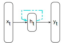This link augments the input to the computation at the hidden layer with the value of the hidden layer from the preceding point in time.

Context: the hidden layer from the previous time step provides a form of memory (context). It encodes earlier processing and is used to drive the decisions at later points in time

This approach does not impose a fixed-length limit on the context. It can include information back from the beginning of the sequence.

RNNs are not all different from non-recurrent architectures.

The most significant change lies in the new set of weights , that connect the hidden layer from the previous time step to the current hidden layer.

The following figure shows that the hidden layer is multiplied by the weight matrix and then added to the feedforward component from the current time step.

We don’t have a fixed lenght window since we process word-by-word and the context can include in principle all information back from the beginning of the text.

Inference in RNNs §

Forward inference (mapping a sequence of inputs to a sequence of outputs) is nearly identical to feedfoward networks.

To compute for an input , the activation value for the hidden layer is needed.

We proceed as in non-recurrent architectures by multiplying the weight matrix with . Morevoer, we multiply the hidden layer from the previous time step with the weight matrix .

Then, these values are addedd together and passed to an activation function .

The usual computation for generating the output vector is used eventually.

• with

is the input dimension, the hidden and the output layer dimension.

A softmax function is used as to get a probability distribution over the possible output classes.

Unrolling an RNN §

The sequential nature i.e the fact that the computation at time requires the value of the hidden layer from time , allows to unroll the network in time:

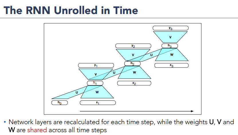
The various layers of units are copied for each time step to illustrate that they will hhave different values over time. However, the various weight matrices are shared across time.

Formally, weight matrices and are fixed because they shared across all time steps. Instead the activation of the hidden layers changes.

Training a RNN §

Like in a feedforward network, we’ll use a training set, a loss function and a back-propagation to obtain the gradients needed to adjust the weights in RNNs

We have 3 sets of weights to update:

• , the weights from the input layer to the hidden layer
• the weights from the previous hidden layer to the current hidden layer
• the weights from the hidden layer to the output layer

Figure: Highlight two considerations:

1. To compute the loss function for the output at time we need the hidden layer from time
2. The hidden layer at time influences both the output at time and the hidden layer at time (and hence the output and loss at )

Therefore, the error due to at each time influences both the current output and the next output that follows.

Training a RNN - Back-propagation through time §

The backpropagation algorithm is a two-pass algorithm for training the weights in RNNs:

1. First Pass: forward inference for computing accumulating the loss at each time step, saving the value of the hidden layer at each step for use at the next time step
2. Second Pass: process the sequence in reverse, computing the required gradients, computing and saving the error term for use in the hidden layer for each step backward in time.

The general approach is called back-propagation through time (Werbos 1974, Rumelhart et al. 1986, Werbos 1990).

With modern frameworks, there is no need for a specialized approach to training RNNs: explicitely unrolling an RNN into a feedforward computational graph eliminates any explicit recurrencies, allowing the network weights to be trained directly.

Note: however for applications that involve much longer input sequences, such as speech recognition, character-level processing, or streamining continuos inputs, unrolling an entire input sequence may not be feasible. So instead, the input is unrolled into manageable fixed-lenght segments and treat each segment as a distinct training item.

RNN as Language Models §

Recall the N-Gram Language Models: it predicts the next word in a sequene given some preceeding context. LM assigns conditional probability to every possible next word, giving us a distribution over the entire vocabulary.

The N-Gram LM computes the probability of a word given counts of its occurrence with the n−1 prior words. The context is thus of size .

For the feedforward (neural) language models, the context is the window size.

RNN as LM: process the input sequence one word at a time, attempting to predict the next word from the current word and the previous hidden state.

RNNs don’t have the limited context problem of n-gram models or the fixed context of feedforward language modele. Since the hidden state can, in principle, represent information about all the preceding words back to the beginning of the sequence.

Difference Between feedforward neural network and RNN: 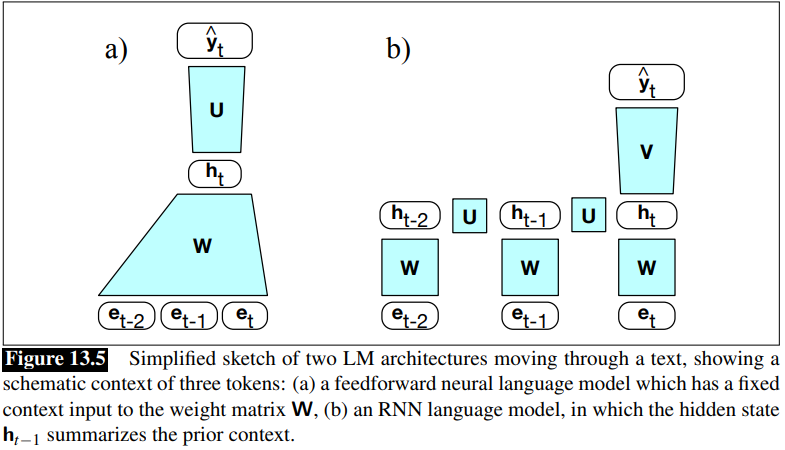The RNN Language model uses , the hidden state from the previous time step, to represent the past context.

Foward Inference in an RNN LM §

The Input Sequence is a series of word each represented as a one-hot vector of size .

The output prediction, is a vector representing a probability distribution over the vocabulary.

At each step:

• the model uses the word embedding matrix to retrieve the embedding for the current word
• multiplies it by the weight matrix
• add it to the hidden layer from the previous step (weighted by weight matrix ) to compute a new hidden layer
• The new hidden layer is then used to generate an output layer which is passed through a softmax layer to generate a probability distribution over the entire vocabulary

At time :

• = softmax()

It is convenient to assume the same hidden and embedding dimensions, (model dimension)

• is
• is
• is
• and are so is
• is so is

The probability that a particular word in the vocabulary is the next word is represented by :

The probability of an entire sequence is just the product of the probabilities of each item in the sequence, where we’ll use to mean the probability of the true word at time step :

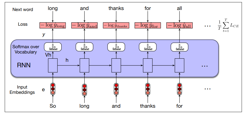
Training an RNN LM §

We use self-supervision (also called self-training): we take a corpus of text as training set and at each time step ask the model to predict the next word.

It is called self-supervised because we don’t have to add any special gold labels to the data; the natural sequence of words is its own supervision!

We train the model to minimize the error in predicting the next true word in the training sequence, using cross-entropy as Loss function, defined as:

the correct distribution comes from knowing the next word (represented as a one-hot vector corresponding to the vocabulary).

So at time the CE loss is the negative log probability the model assigns to the next word in the training sequence:

At each word position of the input the model takes as input three parameters:

• the correct word
• encoding information from preceeding

and uses them to compute a probability distribution over the next words so as to compute the model’s loss for the next token .

Then we move to the next word, ignore what the model predicted for the next word and instead use the correct word along with the prior history encoded to estimate the probability of token .

This idea that we always give the model the correct history sequence to predict the next word is called teacher forcing.

The weights in the network are adjusted to minimize the average CE loss over the training sequence via gradient descent.

The entire process is illustrated in the following figure:

Weight Tying §

Observation: The columns of the embedding matrix are the word embeddings for each word in the vocabulary, learned during the training process.

We assumed as the model dimension.

and have dimension and respectively. This means that the rows of are shaped as the transpose of , meaning that provides a second set of learned word embeddings.

Instead of having two sets of embedding matrices, language models use a single embedding matrix, which appears at both the input and softmax layers ( is used at the start of the computation, and a the end).

This is called weight tying (the same matrix transposed used in two places).

The weight-tied equations for an RNN LM becomes:

This approach provides improved model perplexity and significantly reduces the number of parameters required for the model.

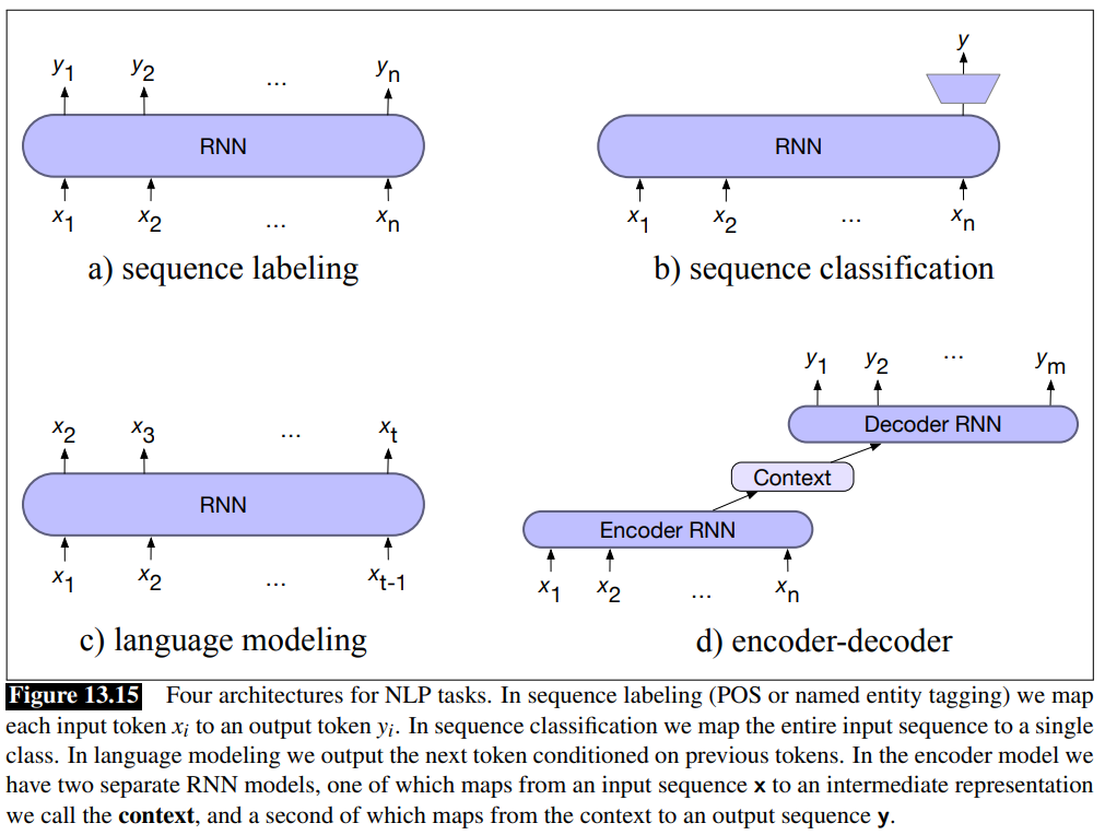
RNN for other NLP Tasks §

The basic RNN architecture can be applied to three types of NLP tasks:

• sequence classification: sentiment analysis and topic classification
• sequence labeling: Part-of-speech Tagging.
• Text generation

RNNs for sequence labeling §

Task: assign a label from a small fixed set of labels to each element of a sequence (e.g., POS tagging and NER) Input: pre-trained word embeddings Output: tag probabilities from a softmax layer over the given tagset

Part-of-speech tagging as sequence labeling with a simple RNN:

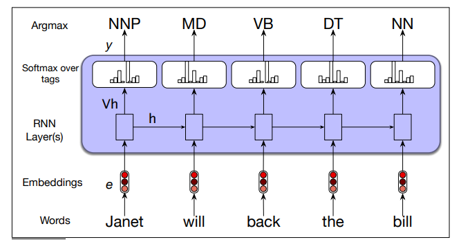
• To generate a sequence of tags for a given input, a forward inference is run over the input sequence, and most likely tag from the softmax is selcted at each step
• cross-entropy loss is used during training.
• Pre-trained word embeddings serve as inputs and a softmax layer provides a probability distribution over the part-of-speech tags as output at each time step.

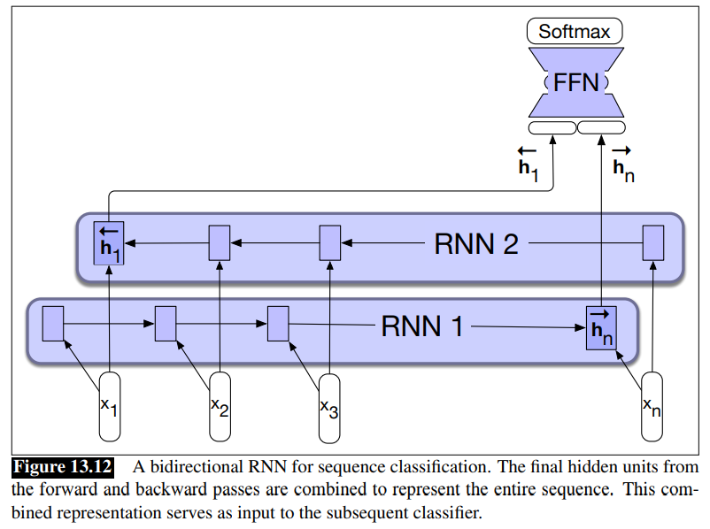
RNNs for sequence classification §

Task: classify entire sequences (text classification) i.e sentiment analysis or spam detection, document-level topic classification.

The text is passed through the RNN one word a time. A new hidden layer representation is generated at each time step. The hidden layer for the last token of the text is token to form a compressed representation of the entire sequence.

This representation is passed to a feedforward network that chooses a class via softmax over the possible classes.

The following figure illustrates this process:

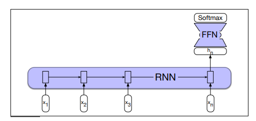
• Sequence classification using a simple RNN combined with a feedforward network. The final hidden state from the RNN is used as the input to a feedforward network that performs the classification.

No loss terms associated with elements before the last. There are no intermediate outputs. The loss function used to train the weights in the network is based entirely on the final text classification. The output from the softmax output from the classifier together with a cross-entropy loss drives the training.

The error from the classification is backpropagated all the way through the weights in the feedforward classifier through, to its input, and then through to the three sets of weights in the RNN (End-to-end training).

Alternatively: it is possible to use some pooling function of all the hidden states for each word in the sequence e.g., element-wise mean:

Generation with RNN-based LMs §

Autoregressive generation: we generate the next word based on which word generated i the previous steps. The same that we overviewed with Neural Network for Text Classification and Language Modelling.

• Initial Word Sampling: Start by sampling a word from the softmax distribution, using the beginning of sentence marker <s> as the first input
• Next Word Input: Use the embedding of the sampled word as input to the network at the next time step and sample the next word from the resulting softmax distribution
• Continue Generation: Repeat this process until the end-of-sentence marker </s> is sampled, or a fixed length limit is reached

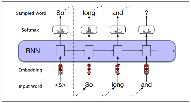
• What we already generated influences what will be generated next.

Technically, an autoregressive model is a model that predicts a value at time based on a linear function of the previous values at time . So we loosely refer to this generation technique as autoregressive generation since the word generated at each time step is conditioned on the word selected by the network from the previous step.

This simple architecture underlies state-of-the-art approaches to applications such as machine translation, summarization, and question answering

Stacked and Bidirectional RNN Architectures §

By combining the feedforward nature of unrolled computational graphs with vectors as common inputs and outputs, complex networks can be treated as modules that can be combined in creative ways.

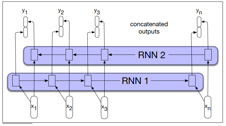
Stacked RNNs §

In a stacked-RNNs the output of one layer serves as the input to a subsequent layer.

• The rationale is that the stacked structure induces representations at different levels of abstraction across layers.
• The optimal number of stacked RNNs is specific to each application and each training set
• However, increasing the number of stacks the training costs rise quickly

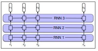
• The output at lower level serves as the input to higher levels
• the output of the last network serves as final output.

Bidirectional RNNs §

Why Bidirectional RNNs Example from Named Entity Recognition:

• He said, “Teddy bears are on sale!”
• He said, “Teddy Roosevelt was a great President!”

If you use a RNN to look at the first part of the sentence to figure that Teddy is part of a person’s name. Because the first three words don’t tell you if they’re talking about Teddy bears or about the former US President.

A bidirectional RNN combines two independent RNN:

• One that process the input from start to end
• The other process the input from end to the start

The two representations from the network are then combined into a single vector that captures both the left and right contexts of the input at each time step.

In the left-to-right RNN that we’ve discussed so far, the hidden state at time is a function of the inputs and represents the context of the network to the left of the current time:

We also train an RNN on a reversed input sequence, so the hidden state at time represents information about the sequence on the right of the current input:

Bidirectional RNN concatenate the two representations:

(We can use also other kind of representation not only concatenation)

The output at each step in time thus captures information to the left and the right of the current input.

• A bidirectional RNN. Separate models are trained in the forward and backward directions, with the output of each model at each time point concatenated to represent the bidirectional state at that time point.

Bidirectional RNNs have also proven to be quite effective for sequence classification.

The Long Short-Term Memory (LSTM) §

• ML2 - Recurrent Neural Networks (RNN) - LSTM and other gated RNNs

RNNs Limitations §

RNNs often struggle to process long-range dependencies.

The information captured in hidden states is typically focues on recent elements, making it difficult for them to consider distant contexts.

This is a significant challenge for many language applications that require understanding distant information. Distant information is critical to many language applications.

Example:

• The flights the airline was canceling were full

Assigning a probability to was is simple since airline is strong local context for the singular angreement.

Conversely, identifying the appropriate agreement for were is challenging because flights is distant, while the singular noun airline appears closer within the intervening context.

A network should be able to retain the distant information about plural flights until it is needed, while still processing the intermediate parts of the sequence correctly.

Vanishing Gradients Problem §

Another difficulty with training RNNs arises from the need to backpropagate the error back through time.

In the backward pass, the hidden layers are subject to several multiplications depending on the lenght of the sequence. The gradients are eventually driven to zero.

The Long Short-Term Memory Extension §

The Long Short-Term Memory (LSTM) was designed to maintain relevant context over time. Enabling to learn to forget information that is no longer needed and to remember information required for future decisions.

LSTM divides context management into two subproblems:

• removing information no longer needed from the context
• adding new information likely necessary for later decisions

LSTM adds to the RNN architeture:

• An explicit context layer (in addition to the usual recurrent hidden layer)
• Specialized neural units that make use of (gates) to control the flow of information into and out of the units that comprise the network layer.
  • In practice, realized by additional weights that work on the input, the previous hidden layer and the previous context layer

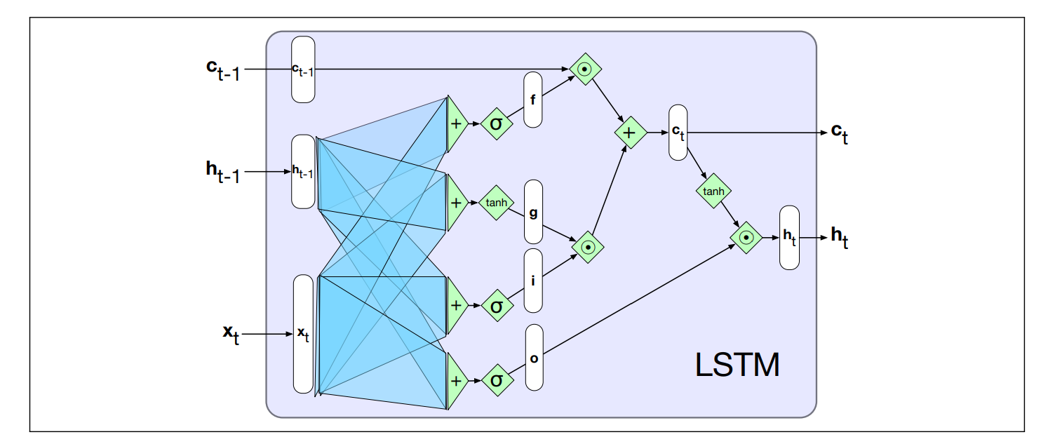
LSTM Gates §

Gate Design Pattern: each gate consists of a feedforward layer, followed by a sigmoid activation function, followed by a pointwise multiplication with the layer being gated.

• Why the sigmoid: push the outputs either to 0 or 1. Combined with a pointwise multiplication has an effect similar to that of a binary mask

Note: the following matrices introduced in the gates are learned during the training process of the network. So for example in the forget gate, the network learns to forget.

Recall: element-wise multiplication of two vectors is the vector of the same dimension as the two input, where each element is the product of element in the two input vectors. **It will be represented by .

Forget gate Removes the information no longer required from the context.

• Takes the previous hidden state and the current input
• Produces a vector of values in
• 1 means “keep this part of the memory”
• 0 means “forget it”

It is applied to the old cell state

Note that during backpropagation, the algorithm should compute that is exatly , but this is approximately so in this way we solve the problem of vanishing gradients.

• The forget gate is upper in the figure, we applied the sigmoid to the previous hidden layer to get , and then we apply it to the previous context layer

Add gate Selects information to add to the current context. This part has two components.

A candidate memory vector:

A filter gate (the gate):

• This decides which part of should actually be added

Then the new information is addedd:

Next, we add this to the modified context vector to get our new context vector:

• using the tanh, the is computed
• applying the sigmoid the filter is computed
• it is then applied to .
• The final cell is updated using the context (that we applied before the remove gate ) and

Output gate What should become the next hidden state?

Decides what the network exposes to the next layer/time-step.

The gate:

Hidden state update:

• Take the current cell state
• Squash it with tanh
• Filter it, using the output gate

This becomes the RNN’s output at time .

• is the current input
• is the previous hidden state
• is the previous context
• Output are a new hidden state and an updated context .

LSTM Cell Output §

The cell state is the long-term memory it carries information across logn sequences with minimal modification. It is passed horizontally through the time to the next LSTM cell .

The hidden state is the short memory, it goes to the next lstm cell (like standard RNN) and to the output layer (when making predictons).

LSTM Modularity §

The complexity of LSTM units is self-contained within the unit.

The only external addition over basic recurrent units is the inclusion of a context vector as both input and output. Modularity to easily experiment with different architectures.

This modularity underpins LSTM’s effectiveness and broad applicability. LSTMs (or variants like GRUs) can be seamlessly integrated into any network architecture. Multi-layer networks with gated units can be unrolled into deep feedfoward networks and trained via standard backpropagation.

Summary of RNN Architectures for NLP Tasks so far §

Transfer Learning: the RNN can be modified to do classification applying another layer at the end.

The Encoder-Decoder architecture with RNNs §

See also:

• ML2 - Lecture 16 - Autoencoders
• Transformers can be used as encoder
• RNN Encoder-Decoder Sequence-To-Sequence Architecture

Why Encoder-Decoder: There are many other applications in NLP where you have to process an input sequence of a length and produce as output of different length. For example, in machine translation you have to produce as output a translation in the target language. And the two sentences in the source and target language are of different length. Another task where there is a similar problem is text summarization.

In all these cases we need the Encoder-Decoder, based on RNNs.

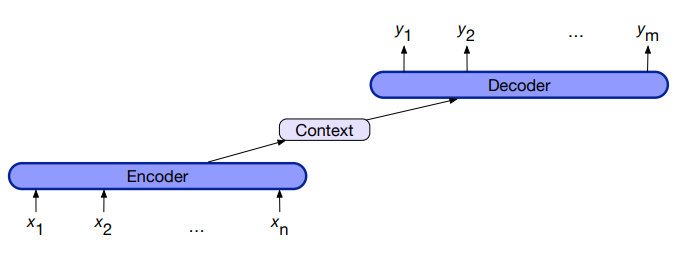
Encoder-Decoder networks (also called sequence-to-sequence networks) generate contextually appropriate, arbitrary-length output sequences given an input sequence.

The key idea is to use:

• an encoder network that takes an input sequence and creates a contextualized representation of it, often called context. (context is a function of the hidden representation of the input)
• a decoder network that takes this representation and generates task-specific output sequence.

• Take an input sequence
• Create a contextualized representation of the input
• Given the input we produce some set of hidden states depending on the lenght of the input sequence.

Encoder-Decoder Components §

1) Encoder that accepts an input sequence and generates the context .

• LSTMs, CNNs, and Transformers can all be used as encoders networks 2) A context vector, , which is a function of
• For example in machine translation could contains all information about the source information 3) Decoder that accepts as input and generates an arbitrary length sequence of hidden states , from which a corresponding sequence of output states is created
• Like for encoders, decoders can be realized by any kind of sequence architecture.

Then the decoder taking information from the context i.e machine translation, generate the output of an arbitrary length.

Encoder-Decor For Translation §

We will see in this section an encoder-decoder network based on a pair of RNNs.

Recall that in any language model, the probability can be breaked down as follows:

If is an activation function like tanh or ReLU and the softmax is over the set of possible vocabulary terms, the output and hidden state at time are computed as:

Sentence separation: We want to translate the source text “the green witch arrived” from engish into spanish “llego´ la bruja verde”

Let be the source text (english sentence) plus a separate token <s>, and the target text (Spanish sentence).

The encoder-decoder model computes the probability

We are computing with the encoder-decoder architecture exactly .

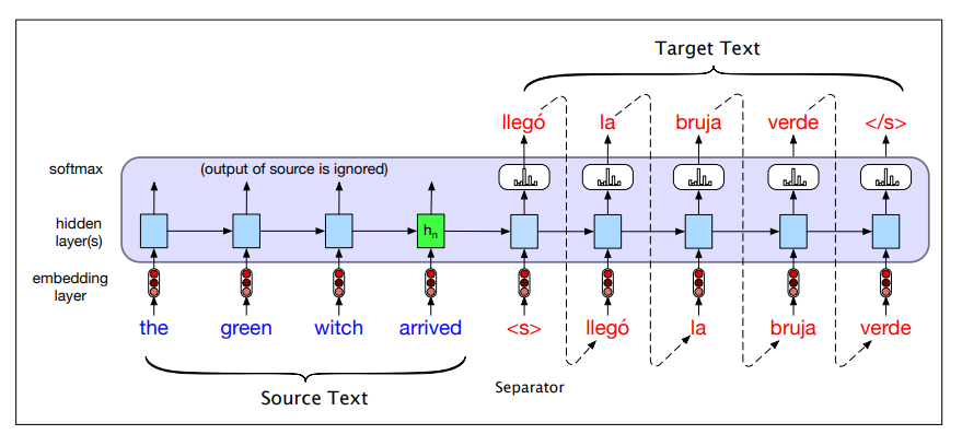
• Source and target sentences are concatenated with a separator token in between
• Decoder uses context information from the encoder’s last hidden state.

Encoder-Decoder Generation Process §

To translate a source text:

1. We run it through the network, performing forward inference to generate hidden states until we get to the end of the source.
2. Autoregressive generation is started
   1. the decoder uses the final encoder hidden state (the summary of the entire source sentence) and the sentence separator as the first inputs.
   2. Subsequent words are conditioned on the previous hidden state and the embedding for the last word generated.

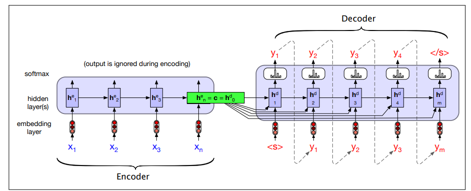
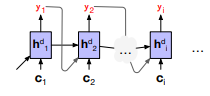
The entire purpose of the encoder is to generate a contextualized representation of the input. This representation is embodied in the final hidden state of the encoder, . This representation is also called for context, is then passed to the decoder.

Whenever we are continuing to produce words, the influence of starts vanishing because we have give it to input just to this one i.e to the node that correspond to the separator.

As shown in figure, what we do is to make the context vector available to more than just the first decoder hidden state, to ensure that the influence of the context vector doesn’t wane as the output sequence is generated.

We do this by adding as parameter to the computation of the current hidden state, using the following equation:

The equations change in this way:

Recall that is a stand-in for some flavor of RNN and is the embedding for the output sampled from the softmax at the previos step.

is a vector of probabilities over the vocabulary, representing the probability of each word occuring at time .

Training the Encoder-Decoder §

The training procedure is end-to-end. Each training example is a tuple of paired strings, a source and a target, concatenated with <s>. For MT, the training data typically consists of sets of sentences and their translations.

Training is shown in the following figure:

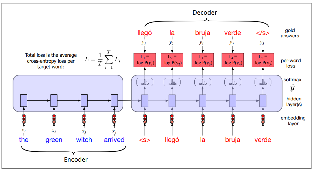
• In the autoencoder we don’t propagate the model’s softmax output but use teacher forcing to force each input to the correct gold value for training
• Then compute the softmax output distribution over in the decoder in order to compute the loss at each token, which can then be averaged to compute a loss for the sentence.
• This loss is then propagated through the deocoder parameters and the encoder parameters.

Training vs Inference differences: decoder during inference uses its own estimated output as the input for the next time step . Thus the decoder will tend to deviate more and more from the gold target sentence, as it keeps generating more tokens. In training, it is more common to use teacher forcing in the decoder, forcing the system to use the gold target token from training as the next input , rather than allowing it to rely on the (possibly erroneous) decoder output . This speeds up training.

When we compute the loss instead of computing the loss of best predict we compute the loss associated with each golden label.

Once the training set is prepared, the RNN-based language model is trained autoregressively. The network takes the source text, starts from the separator token, and predicts the next word (teacher forcing).

This procedure makes the training process faster.

This is done at both level, encoder and decoder, you can use complex architecture. So for example stacked RNNs and so on.

Attention §

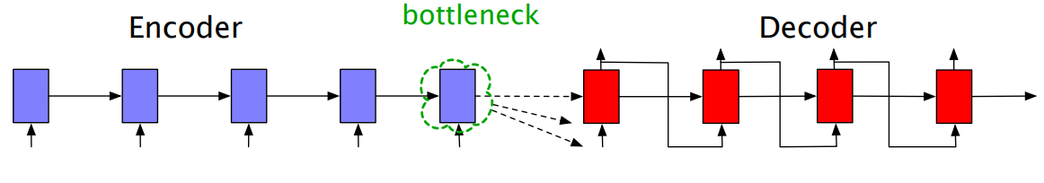
Bottleneck problem We’ve just seen that the context vector is the hidden state of the last time step of the source text. is acting as a bottleneck: it must represent everything about the meaning of the source text, since the only thing the decoder knows about the source text is what’s in this context vector. Information at the beginning of the sentence, especially for long sentences, may not be equally well represented in the context vector.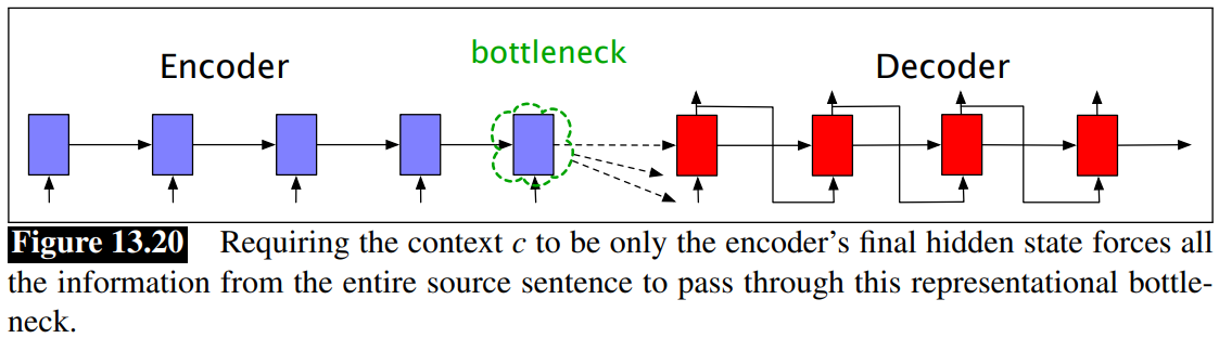

We don’t want to consider only but all the hidden states of the encoder i.e and exploit the most relevant parts. In this way we have a more precise representation of the meaning of the source sequence. However i don’t know hwo many hidden states i have because the encoder has a number of hidden state that corresponds to the length of the sentence but we don’t know the length of the sentence.

Attention Mechanism: The attention mechanism is a solution to the bottleneck problem. It allows the decoder to get information from all the hidden states of the encoder.

In the attention mechanism, the context vector is a single vector that is a function of hidden states of the encoder:

• means hidden state of the encoder

The idea is to create a single fixed-length vector by taking a weighted sum of all the encoder hidden states.

The weights focus on a particular part of the source text that is relevant to the token the decoder is currently producing.

Attention replaces the static context vector with one that is dynamically derived from the encoder hidden states, different for each token in decoding.

The context vector is generated at each decoding step and is derived by considering all the encoder’s hidden states. This context is then available during decoding by conditioning the computation of the current decoder hidden state on it (along with the prior hidden state and the previous output generated by the decoder). This is represented by this equation:

And shown in this figure:

Dot-product attention The first step in computing is to compute how much to focus on each encoder state, that is, how relevant each encoder state is to the decoder state captured in .

The relevance is captured by computing, at each state i during decoding, a score as a similarity (dot-product attention)

The result is a scalar that reflects the degree of similarity between the two vectors.

The vector of scores across all the encoder hidden states provides the relevance of each encoder state to the current step of the decoder.

A vector of weights, , is created by normalizing the vector of scores:

Finally, given the distribution , we can compute a fixed-lenght context vector for the current decoder state by taking a weighted average over all the encoder hidden states.

• is simply the weighted average over all the encoder hidden states

With this, we have a fixed-length context vector that captures information from the entire encoder states, dynamically updated at each decoding step.

Next figure shows a sketch of the encoder-decoder network with attention, focusing on the computation of .

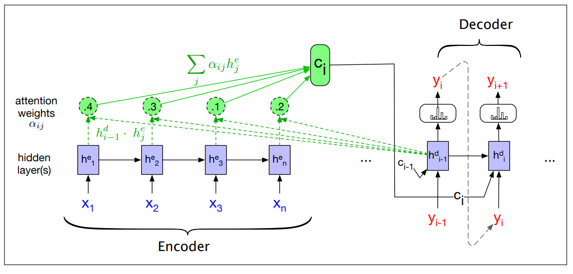
• We first compute alle the encoder states
• Then we can compute the similarity and get
• The context value is one of the inputs to the computation of . It is computed by taking the weighted sum of all the encoder hidden states, each weighted by their dot product with the prior decoder hidden state
• that becomes also input of the decoder.
• When computing and we are taking into account part of the content that is relevant to produce this output, and this is dynamic since changes for all the states of the decoder because they are computed at the basis of similarity of the previous activation.

More sofisticated scoring functions: It’s also possible to create more sophisticated scoring functions for attention models. Instead of simple dot product attention, we can get a more powerful function that computes the relevance of each encoder hidden state to the decoder hidden state by parameterizing the score with its own set of weights,

The weights , which are then trained during normal end-to-end training, give the network the ability to learn which aspects of similarity between the decoder and encoder states are important to the current application.

This bilinear model also allows the encoder and decoder to use different dimensional vectors, whereas the simple dot-product attention requires that the encoder and decoder hidden states.

A slight modification of attention, called self-attention is the basis on the [[NLP - Lecture - Transformers for NLP|[NLP] Transformers]] architecture.

---