NLP - Lecture - Machine Translation

---

NLP - Lecture 14 - Machine Translation §

Given a word in a source language, we can predict its equivalent in a target language. We consider the simpler case where we only translate words and not an entire translated sentence.

The idea is to use word vector representations to learn a mapping between languages. For example, given English and French word embeddings, the goal is to map each English vector to its French counterpart.

This mapping can be learned using any word representation, from bag-of-words or TF-IDF to word embeddings seen in previous lessons.

Overview of translation §

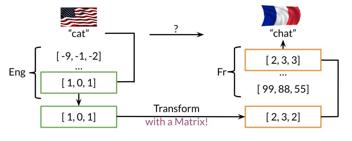
Suppose we want to make a English to French translation.

Generate an extensive list of english words and their associated french words.

1. Compute the word embeddings associated with english and word embeddings associated with french
2. Retrieve the english word embedding of a given english word
3. Find a way to transform english word embedding into the same meaning french word embedding by learning a transformation matrix
4. Search for word vectors in the french word vector space that are most similar to the transformed english word embedding (the most similar words are candidates’ words for the translation)

Transforming vectors §

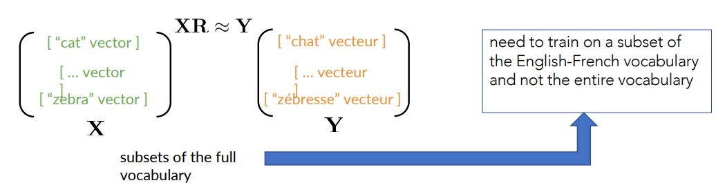
We have to find the matrix that make possible to transform english vectors into correspoding French vectors

Formally

Let’s start by a random matrix

We first need to get a subset of english words and their french equivalent. Then get their respective word vectors and stack the word vectors in the respective matrices, and . It’s mandatory to align the word vectors.

Finding a good R §

Define a loss function to measure the ”quality” of the translation (transformation) w.r.t the actual French words (vectors).

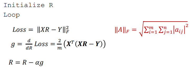
Starting with a random , we can iterate for the optimal using the gradient descent

1. Initialize
2. Loop:
   1. Loss =
   2. g = derivate of the loss function

where is the learning rate. It’s the classical gradient descent.

Frobenius Norm: measures the magnitude of a matrix

We apply as our criterion the square of so we remove the square root during the computing of frobenius norm.

If we apply some computations to the loss the gradient becomes:

Optimizing R §

K-Nearest Neighbors §

With the previous method i find the transformation matrix . But how do i use this transformation matrix in order to, given a word in english, compute the corresponding one in french?

I could use the cosine similarity for searching the closest vector. However, it’s computationally intensive.

The K-NN can be used to efficiently find the most similar word to the one transform in the destination language.

K-NN Intuition and Hash Tables §

K-NN Intuition 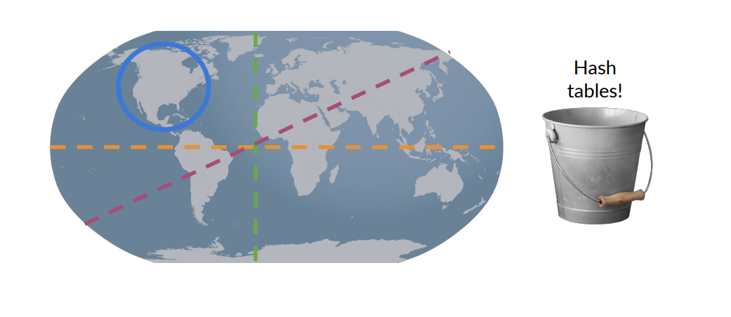Suppose we have several data items and we want to group them into buckets by some kind of similarity

One bucket can hold more than one item, and each item is always assigned to the same bucket.

Finding the Translation §

A way to find a matching word after the transformation is to use k-nearest neighbours.

After a transformation through the matrix , a vector is in the French word vector space:

• is not necessarily identical to any word vector in the french vector space.
• One need to search through the actual french word vectors to find a similar word

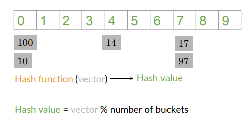
Hash function §

We can do the same with word vectors: assuming that the word vec have just one dimension, so each word is represented by a single number such as 100,14,17,10 and 97.

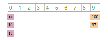
A function (hash function) assigns a hash value:

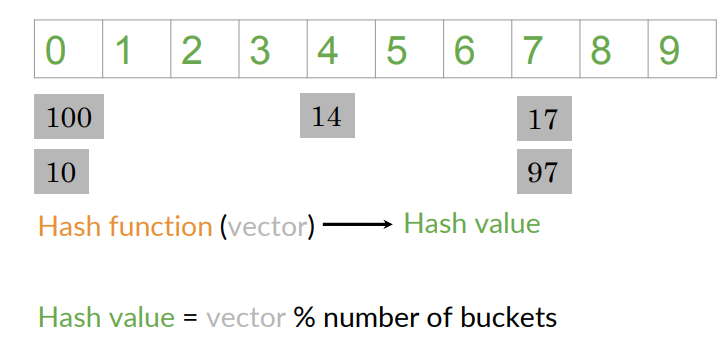
Ideally, this hash function should put similar word vectors in the same buckets.

Locality Sensitive Hashing §

Locality sensitive hashing: a method that assigns items based on where they’re located in vector space.

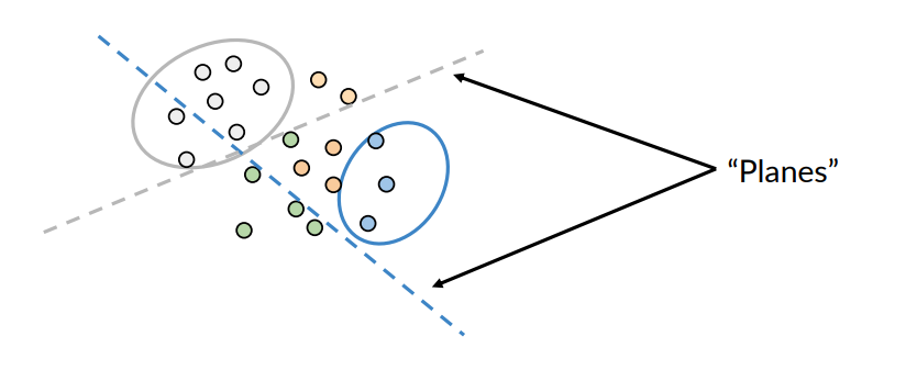
To build LSH, let’s introduce the idea of planes (hyperplanes)

Each plan divides the space into two halves:

• the blue plane divides the space with blue vectors above it
• the grey vectors area above the gray plane

The plane helps us put the vectors into subsets based on their location

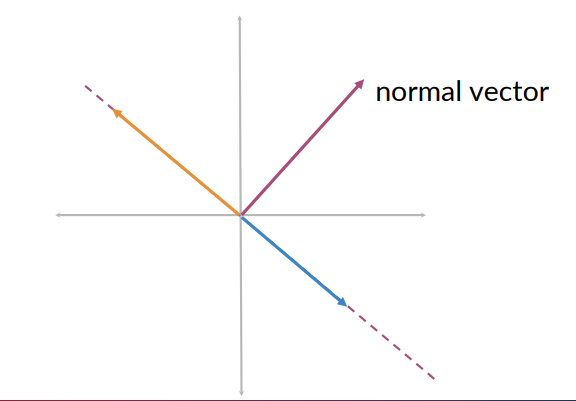
Planes §

A plane represents all the possible vectors lying on that plan (e.g., the blue or orange vectors). Each plane is defined by a normal vector (magenta vector):

• It is perpendicular to any vector that lie on the plane
• Mathematically, it gives the orientation of the plane in space.

Finding the side of the plane §

How do we find the side of the plane where a vector lie, mathematically? Consider the dot product.

Knowing the normal and a point , the dot product determines on which side of the plane the point lies.

When

• the dot product is positive, the vector is on one side of the plane
• If the dot product is negative, the vector is on the opposite side of the plane
• If the dot product is zero, the vector is on the plane

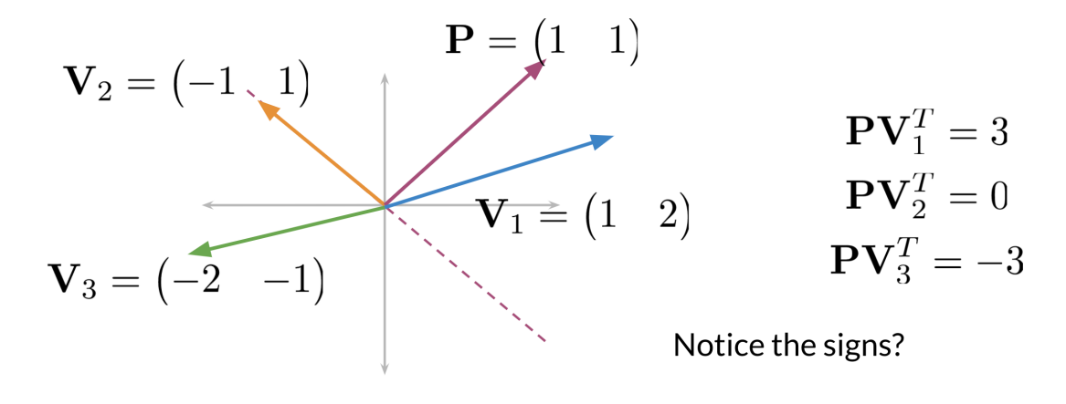
Let’s focus on single vector 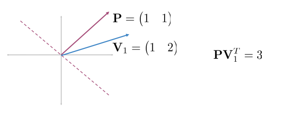: Now consider the other vectors:

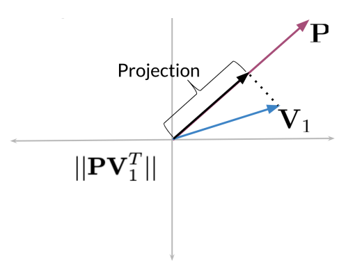
Visualizing a dot product §

Consider the plane represented by vector P

• The dot product between P and is a positive number
• It’s the length of the projection of onto

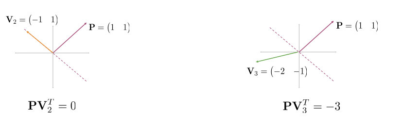
The green vector projected onto , points on the parallel and opposite direction of .

The dot product is a negative number

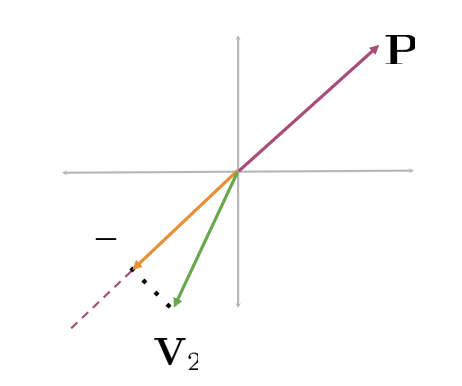
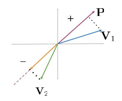
The sign of the dot product indicates the direction of the projection with respect to the normal vector

• If it is positive or negative tells us whether the vectors or are on one side of the plane or the other
• The sign indicates the direction

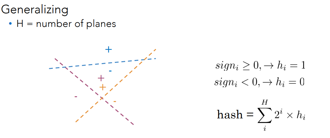
Multiple Planes §

How do we get a single hash value from multiple planes? i.e., identify where a data point is given several planes.

We aim at dividing the vector space into manageable regions

• Goal: determining a single hash value identifying a particular region within the vector space

Each planes gives a binary decision:

Having 3 planes, each one contributes one bit. All together they provide an 3-bit binary code.

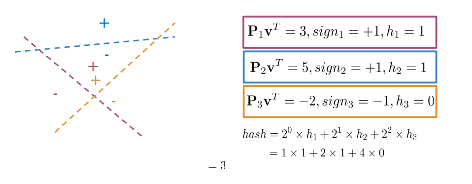
By applying this rule, each word is placed into a specific bucket. This allows us to search only within that limited region, greatly reducing the search space. Instead of comparing against, say, 300,000 points, we now look at only about 100. Within this smaller bucket, we can then compute similarities — for instance, using cosine similarity — to find the most similar word efficiently.

There is a tradeoff: choosing :

• Too few planes -> too many vectors per bucket (less precision)
• too many planes -> too many empty buckets (inefficinet lookup).

Approximate K-NN §

These planes are randomly generated because as we know the initialization of k-NN is random.

Even with one set of planes, one might miss neighbours near the boundary of a plane.

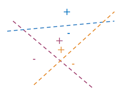
Idea - create multiple sets of random planes:

• Multiple independent sets of hash tables
• When searching, the candidate buckets from all the tables are searched.

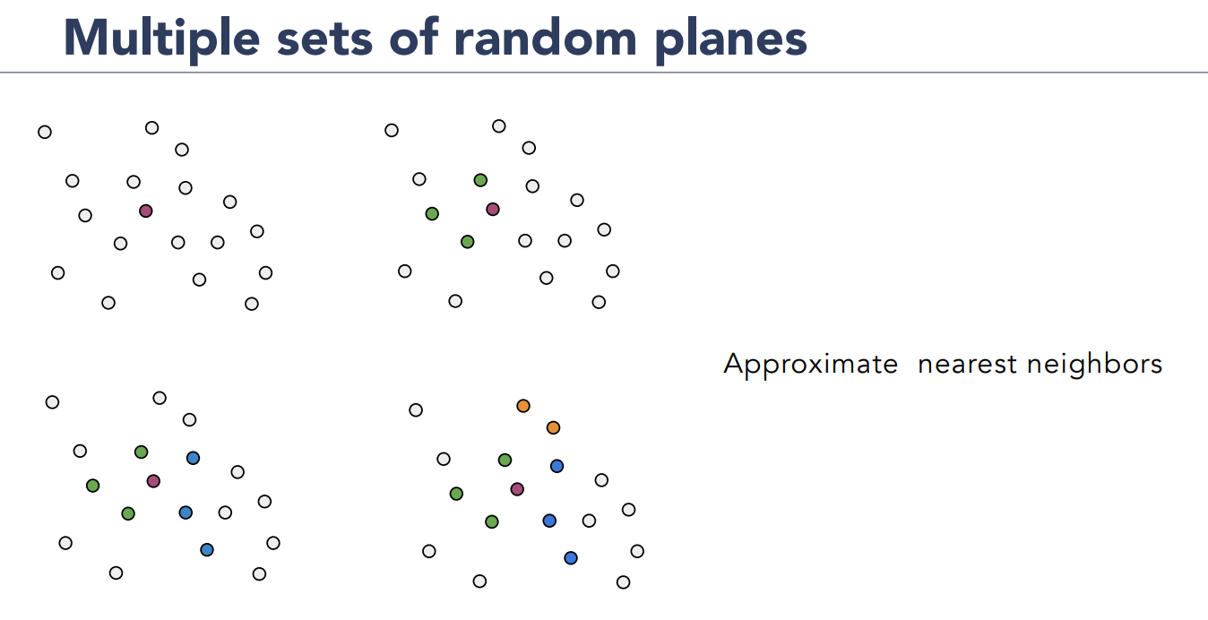Say that we get the point (purple up-left). let’s say that these greens (up-right) are one bucket. Then we generate another set of planes randomly, and we could have that green and blue goes into different bucket (bottom-left) and so on.

Approximate nearest neighbors:

• Do not guarantee to find the absolute closest neighbour (expensive)
• Accept a very close one that’s much faster to find
• This small loss in accuracy leads to a huge gain in efficiency

How do we use approximate KNN in practice? §

1. generate random planes: defined space partition
2. initialize hash tables: one per random partition
3. Compute hash code for each vector: binary encoding per table
4. Insert vector index in bucket: groups similar vectors
5. Repeat for multiple tables: improve recall
6. Store as dictionaries: efficient lookup at query time.

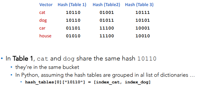
Each table will be a dictionary that maps:

• Hash code list of indices of vector
  • For example if a vector gets hash code 101010 that string will be the key.
  • The hash value will be a list of indices of vectors that share that hash

How to compute a hash code:

• For each vector :
  • We project it on every plane:
  • Assign bit if else 0
  • Then we concatenate those bits to form a hash string, like 101010

Example: Bucket Computation

Assume of having four planes (four normal vectors), :

• Projections on planes: (dot product )
• Signs:
• Hash bits:
• Final code:
  • That is, is in bucket for this table

Searching Documents §

What it is said before can be also applied for search inside documents.

Let’s represent a document as vector, we have different method to do this like word embedding.

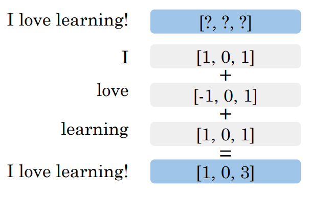
If i do this, given a document, represented as a vector, i can apply exactly the same idea of approximating K-NN in the problem of searching the most similar one document or words.

We have multiple ways to represent documents as vectors, as we discussed in the previous lesson (Bag Of Words, Average Word Embeddings, Doc2Vect/sentence transformerd, encoder from large models).

Doc2Vec is interesting bcs it learns direct mapping from text to embedding (trained neural models) Large models use the hidden representation of the document from a pretained transformer.

Document search §

Once each document is represented as a vector:

• A query is also converted into a vector
• Use K-NN to find the closest document vectors to this query vector
• The closest documents are returned as the most relevant ones

This is the same principle as for machine translation we’re just applying it to documents instead of words.

---