NLP - Lecture - Transformers for NLP

---

NLP - Lecture - Transformers §

• 8.pdf

In the previous topic, attention in sequence models we introduced attention. Transformers are based on these, but employs self-attention.

First, left-to-right (also called casual or autoregressive) language modeling is introduced through transformers.

Attention can be thought as building contextual representations of a token’s meaning by attending to and integrating information from surrounding tokens.

Recall that in [[NLP - Lecture - Static Word Embeddings|[NLP] Word Embeddings]], we talked how algorithms like word2vec produce static embeddings. Also neural network can learn from data and produce static embedding. A static embedding DOESN’T reflect how it meaning changes in context. Transformers can compute dynamic embeddings that solves this problem, called contextual embeddings.

Big Picture

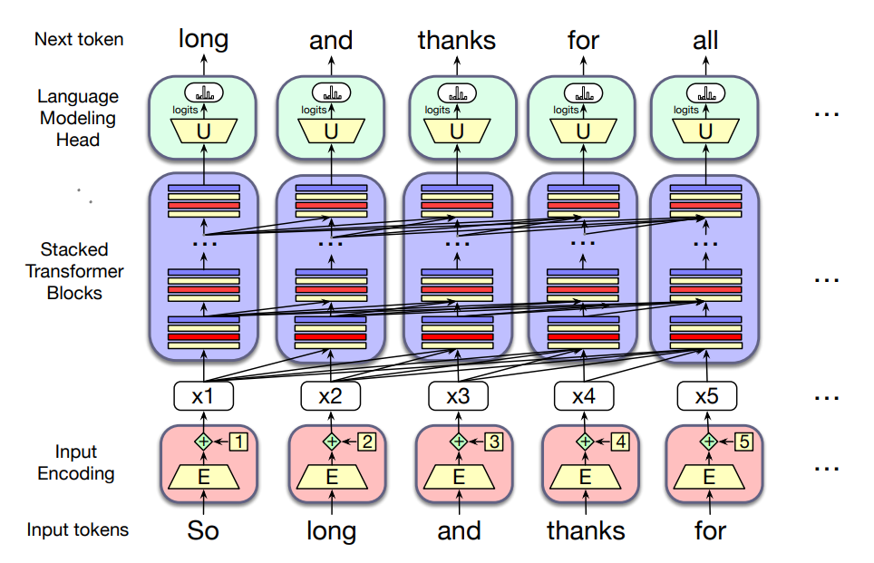
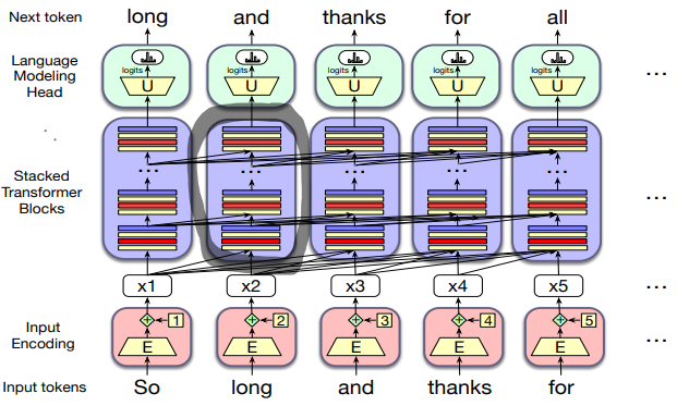
• This figure sketches the transformer architecture
• Three major components
• At the center there are columns of transformer block, each one is a multilayer network (a multi-head attention layer, a feedforward network and a layer normalization steps) that maps an input vector in column (corresponding to input token to an output vector ).
• The set of blocks maps an entire context window of input vectors to a window of output vector of the same length.
• Input encoding component: processes an input token (like the word thanks) into a contextual vector representation using an embedding matrix and a mechanism for encoding token position.
• Each column is followed by a language modeling head, which takes the embedding output by the final transformer block, passess it through an unembedding matrix and a softmax over the vocabulary to generate a single token for that column.

Attention §

Contextual Embeddings §

Let’s consider the embeddings for an individual word from a particular layer.

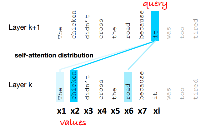
Example: The chicken didn’t cross the road because it was too tired.

What is the meaning represented in the static embedding for “it”?

Intuition: a representation of the meaning of a word should be different in different contexts.

In contextual embedding, each word has a different vector that expresses different meanings depending on the surrounding words.

To compute contextual embeddings, attention is used.

In the sentence: “The chicken didn’t cross the roat because it…” What should be the properties of “it”?

• The chicken didn’t cross the road because it was too tired
• The chicken didn’t cross the road because it was too wide

In the first sentence, the reader knows that it’s the chicken that it’s tired, and in the second, it’s the road that it’s wide. But a casual language model with a left-to-right architecture wouldn’t necessary understand this.

Overview of attention §

Attention builds up the contextual embedding form a word by selectively integrating information from all the neighbouring words.

A word “attends to” some neighbouring words more than others.

Attention is formally defined as: the mechanism in the transformer that weighs and combines the representations from appropriate other tokens in the context from layer to build the representation for tokens in layer .

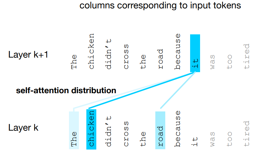
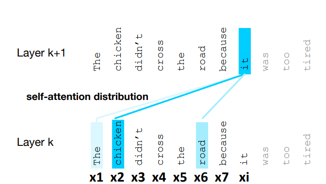
• Figure shows the self-attention weight distribution that is part of the computation of representation for the word it at layer
• In computing the representation for it, we attend differently to the various words at layer k, with darker shades indicating higher self-attention values.

Simplified Attention §

Input:

• representation corresponding to the input token at position ,
• context window of prior inputs

and produces an output .

Information flow in casual self-attention: it is left-to-right, this means that the context is any of the prior words. When processing , the model has access to the representation of and also the representations of the prior tokens in the context window (usually thousands of tokens), but no tokens after .

Seeing tokens after is a characterstic of Masked Language Models.

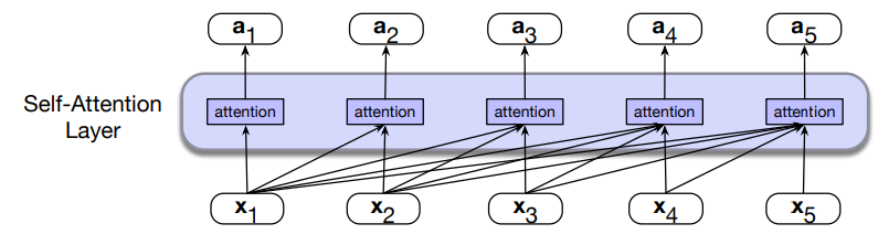
Ofcourse, the same attention computation happens in parallel at each token position .

A self-attention layer maps input sequences to ouput sequences of the same lenght .

Simplified version of attention: consider first a simplified intuitive version of attention, in which the attention output (token position ) is simply the weighted sum of all the representations for all : Simplified version: .

is a scalar used for weighting the value of input when summing up the inputs to compute . So the problem becomes how to compute this weight.

In attention we weight each prior embedding proportionally to how similar is it to the current token . So the output of attention is a sum of the embeddings of prior tokens weighted by their similarity with the current token embedding. Defined through a similarity score, via dot product:

The larger the score, the more similar the vectors that are being compared. Then the scores must be normalized with a softmax to create the vector of weights :

and

Intuition of Attention: so we compute by computing three scores: , normalizing them by softmax and using the resulting probabilities as weights indicating each of their proportional relevance to the current position .

Attention Head §

Head in transformers is used to refer to specific structured layers

instead of using vectors like (and ) directly, each input embedding plays three separate roles:

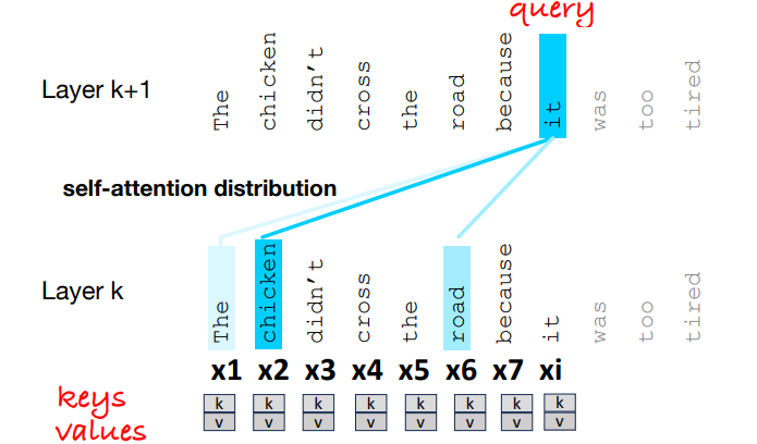
• Query: when the vector is the current element being compared to the preceding inputs
• Key: the vector is the preceding input that is compared to the current element to determine a similarity
• Value: the value of a preceding element that gets weighted and summed up to compute the output for the current element

To capture these three different roles, transformers introduce weight matrices:

• query:
• key:
• value:

These weights will projct each input vector into a representation of its role as a query, key or value:

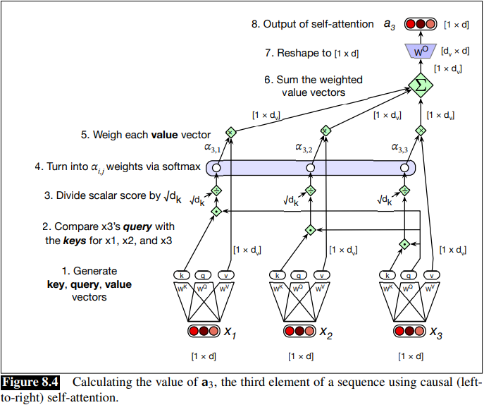
Given the three representation of . To compute the similarity of the current element with some prior element :

• It is considered the dot product between the current element’s query vector and the preceding element’s key vector

Attention weight, score and output: The attention weight between token and is computed by doing . This give us one information: which tokens matter for producing the next representation. But this score says nothing about what information to extract. Values determine what content is passed forward, therefore the output will be given by . Values are learned through .

Another issue, is that the dot product can be a arbitrarily large (positive or negative) value, and exponentiating large values can lead to numerical issues and loss of gradients during training, so it is normalized by the square root of . The factor is choiced as related to the size of the embeddings.

Softmax calculation resulting in remains true, but it is multiplied by instead of .

Final set of equations for computing self-attention for a single self-attention output vector from a single input vector :

Model Dimensionality and why the matrix The matrix is right-multiplied by the attention head, and is used to reshape the output of the head. The input to attention and the output from attention have the same dimensionality , is called model dimensionality. The output of each transformer block also have the same dimensionality . Having everything be the same dimensionality makes the transformer very modular.

This is more or less the chain:

1. are both so it becomes a scalar
2. is the dimension for value vectors choosen arbitrarily (i.e in original paper 64) and is the dimension of value vectors.
3. and has shape , while is
4. The output head has shape .
5. TO get the desired output shape ], a matrix is of shape ]

On the Value Role: We don’t use the raw token embeddings as values because:

• Different attention heads need different transformed information from each token, not just the original embedding
• The model learns which aspects of a token should be “copied forward” once attention decides it is important
• Values allow separation between how strongly we attend to a token and what information we take from it .

Multi-head Attention §

Idea: instead of one attention head, we ‘ll have a lot of them.

Example: suppose the sentence is “The bank raises interest rate”, different attention heads may want:

• syntactic info (noun: subject)
• semantic info (bank: financial institution)
• contextualized info (economic topic)

Using directly the value, every head gest the same representation of “bank”, so they cannot specialize.

Intuition: each head might be attending to the context for different purposes, some may specialized to represent different linguistic relationships between context elements and the current token, or to look for particular kinds of pattern in the context.

Multi-head attention: we have a number of separate attention heads that reside in parallel layers at the same depth in a model, each with its own set of parameters that allows the head to model different aspects of the relationships among inpus.

Each head in a self-attention layer has its own set of query, key and value matrices: , and . Each matrix is used to project the inputs into separate query, key and value embeddings for each head.

Model dimensionality of multi-head: is still used for input and output, for value embeddings and for query and key embeddings as before.

Equations for attention augmented with multiple heads:

• MultiHeadAttention() =

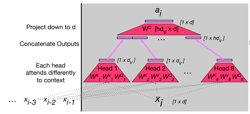
The output of each of the heads is of shape ], so the output of the multi-head layer with heads consists of vectors of such shape. These are concatenated to produce a single output with dimensionality . Then we use yet another linear projection to reshape it, resulting in the multi-head attention vector with the correct output shape at each input .

The Transformer Block §

The self-attention calculation lies at the core of what’s called a transformer block, which, in addition to the self-attention layer, includes three other kinds of layers:

1. a feedforward layer,
2. residual connections,
3. normalizing layers (colloquially called “layer norm”)

A common way of thinking about the block: the residual stream i.e each token gets passed up and modified.

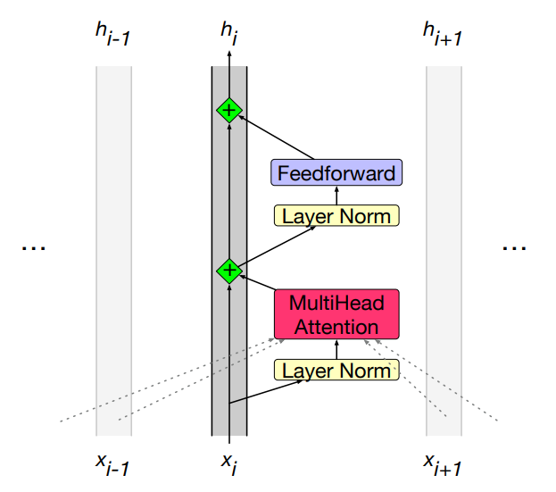
• Figure shows the residual stream: the prenorm version of the architecture, in which the layer norms happen before the attention and feedforward layers rather than after.

Feedforward layer: The feed-forward layer is a fully-connected 2-layer neural network with one hidden layer and two weight matrices. It provides us with the needed nonlinearities:

While attention mixes information across tokens, FFN operates independently on each token:

• Refines each token representation individually
• Helps the model encode local features and non-contextual properties
• Stabilises token embeddings after attention mixing

This allows the transformer to approximate more complex functions and decision boundaries.

Overall

• Attention tells the model what to look at
• The FFN tells the model how to transform what it found

Layer Norm The layer norm is a variation of -score from statistics applied to a single vector in a hidden layer. Note: norm isn’t applied to the entire layer but just to the embedding vector of a single token. First we compute mean and standard deviation over the elements of the vector to be normalized:

Then the vector components are normalized by subtracting the mean from each and dividing by the standard deviation:

Finally, two learnable parameters and representing gain and offset values are introduces:

Putting together a single transformer block §

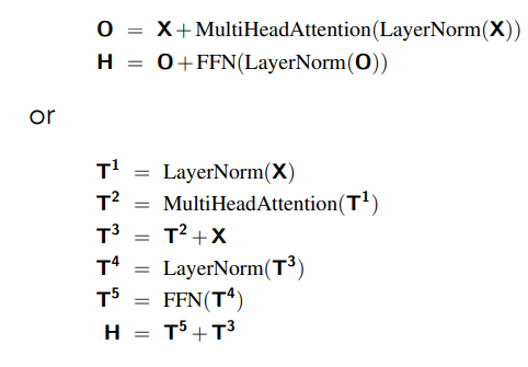
The function computed by a transformer block can be expressed by breaking it down with one equation for each component computation, using 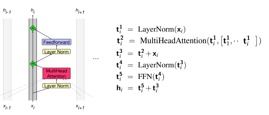of shape to stand for transformer, superscripts to demarcate each computation inside the block:

Stack of blocks: a transformer is a stack of these components. All vectors are of the same dimensionality . The number of stacked blocks ranges from 12 to 96.

One more requirement: at the very end of the last (highest) transformer block, there is a single extra layer norm that is run on the last of each token stream (just below the language model head layer).

Residual Streams Attention heads can be seen as moving information from the residual stream of a neighboring token into the current stream.

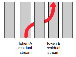
Notice that the only component that takes as input information from other tokens (other residual streams) is multi-head attention, which (as we see from equation) looks at all the neighboring tokens in the context.

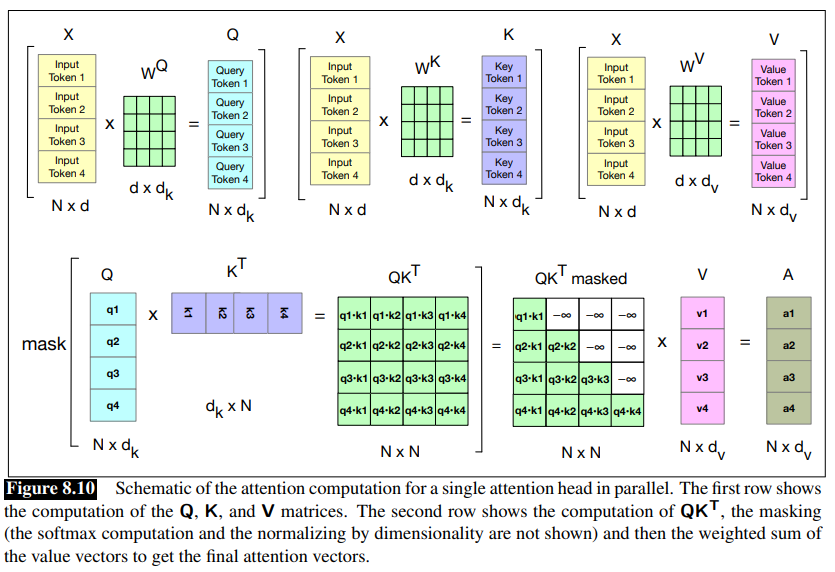
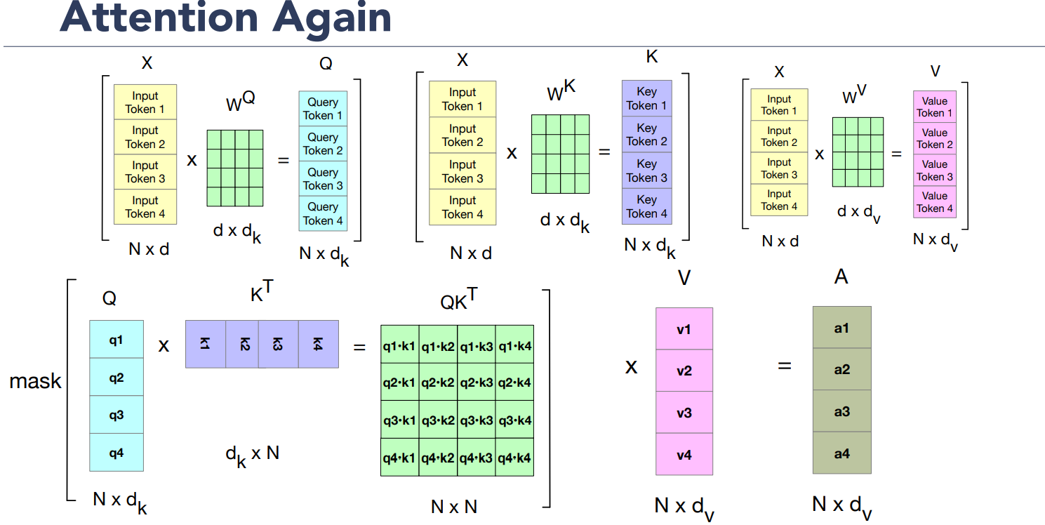
Parallelizing Attention §

The attention computation performed for each token to compute is independent of the computation for each other token, and that’s also true for all the computation in the transformer block computing from the input . That means we can easily parallelize the entire computation, taking advantage of efficient matrix multiplication routines

But we can pack the input embeddings for the tokens of the input sequence into a single matrix of size . Each row of is the embedding of one token of the input.

can have 1K-32K rows, each of dimensionality of the embedding d (the model dimension).

Parallelizing Attention - Single Head Attention. For one head we multiply by the query, key and value matrices of shape , of shape ] and of shape , to produce matrice of shape , of shape ] and of shape containing all the key, query and value vectors:

We can compute all the requisite query-key comparisons simultaneously by multiplying 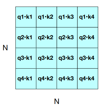and in a single matrix multiplication. (Note: only a single matrix multiplication is needed). The product is shown in this figure:

Once we have the matrix, the scores can be very efficiently scaled, take the softmax and multiply by , resuing in a matrix:

Masking out the future We introduced a mask function, because the self-attention has a problem: it cheats by looking at the future and including key-value that follows the token in the query. 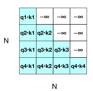Guessing the next word is simple if you already know it. Solution: add to cells in the upper triangle (the softmax will turn it to 0).

Observation: attention is quadratic in lenght.

Parallelizing Multi-Head Attention The model has:

• a dimension
• query and embeddings have dimensionality
• value embeddings are of dimesionality

For each head , we have we have weight layers:

• of shape
• of shape
• and of shape

These get multiplied by the inputs packed into to produce:

• of shape ],
• of shape
• and of shape .

The output of each of the heads is of shape and so the output of the multi head layer with heads consists of matrices of shape . To make use of these matrices in further processing, they are concatenated to produce a single output with dimensionality . Finally, a linear projection of shape reshapes it to the original output dimension for each token.

Putting it all together with the parallel input matrix : the function computed in parallel by an entire layer of transformers blocks, each block over one of the input tokens, can be expressed as:

• by we mean the input to the layer, wherever it comes from. For subsequent layers , the input is the output of the previous layer .
• In the second part of equations, the computation performed by a transformer layer are breakd down, showing one equation for each component. stands for transformer and superscripts denote each computation inside the block.

Input: embeddings for token and position §

Given a sequence of tokens ( is the context length in tokens), the matrix (of shape ) has an embedding for each word in the context. The transformer creates this embedding by separately computing two embeddings: an input token embedding, and an input positional embedding.

The set of initial embeddings are stored in the embedding matrix has a shape :

• One row for each of the tokens in the vocabulary
• Each word is a row vector of dimension

Example: Given an input string ”Thanks for all the“:

1. Convert the tokens into vocabulary indices (created when we first tokenized the input using BPE or SentencePiece), so the representation might be
2. Select the corresponding rows from , each row an embedding: (row 5, row 4000, row 10532, row 2224)

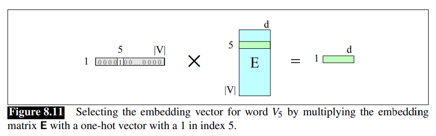
Another way to think about selecting token embeddings from the embedding matrix is to represent tokens as one-hot vectors of shape i.e. with one dimension for each word in the vocabulary.

Recall that in a one-hot vector all the elements are 0 except one, the element whose dimension is the word’s index in the vocabulary, which has value 1.

This can be extended to represent the entire token sequence as a matrix of one-hot vectors, one for each of the 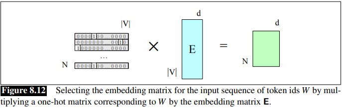positions in the transformer’s context window:

Positional Embedding §

These token embeddings are not position-dependent. To represent the position of each token in the sequence, we combine these token in embeddings with positional embeddings specific to each position in an input sequence.

Transformers process text as a sequence of tokens. However, unlike RNNs, they do not inherently know the order of tokens.

To fix this, they add positional information to each token’srepresentation, therefore

• Token embedding tells the model what a word is (e.g., “fish”).
• Positional embedding tells the model where the word is located in the sentence (e.g., 3rd position, 17th position, etc.)

To represent the position of each token in the sequence: combine token embeddings with positional embeddings specific to each position in an input sequence.

There are many methods, but we’ll just describe the simplest: absolute position, shown in the figure:

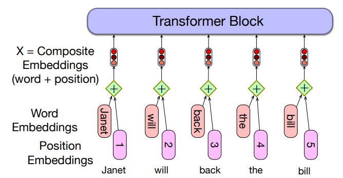
Start with randomly initialized embeddings

• one for each integer up to some maximum length
• i.e., just as we have an embedding for token fish, we’ll have an embedding for position 3 and position 17

As with word embeddings, these positional embeddings are learned along with other parameters during training. Then they are stored in a embedding matrix of shape .

The final representation of the input, the matrix is an matrix in which each row is the representation of the th token in the input, computed by adding , the embedding of the id of the token that occured at position , to , the positional embedding of position .

Absolute Positional Embedding Issues: In absolute positional embedding, we treat positions like a vocabulary of words. We define a maximum sequence length and for every integer we learn a unique vector .

These embeddings are learned during training, just like word embeddings. For instance, if the model is trained with it physically cannot process a sequence of 513 tokens.

Another issue is with data, during training most sentences are short:

• So early positions (like ) appear very often, but positions near the maximum length appear rarely
• Embeddings for long positions may be low quality and may not generalize.

Alternatives Positional Encodings

In the original transformer work, a static function as a combination of sine and cosine functions with different frequencies is used.

Sinusoidal position embeddings may also help in capturing the inherent relationships among the positions, the fact that position in an input is more closely related to position than it is to position .

Another option is to represent relative position instead of directly absolute position. Often implemented in the attention mechanism at each layer, rather than being added once at the initial input.

Output: The Language Modelling Head §

(Language Model) Head means the additional neural circuitry that is added on top of the basic transformer architecture when we apply pretrained transformer model to various tasks.

Recall NLP - Lecture - Language Models, N-Grams, Perplexity and how they work. A language models allow, given a context of words (context window) to assign a probability to each possible next word.

Transformers context is represented through a a context window, which can be quite large, like 32K tokens for large models.

The job of the language modeling head is to take the output of the final transformer layer from the last token N and use it to predict the upcoming word at position N +1.

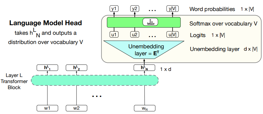
• The circuit at the top of a transformer that maps from the output embedding for token from the last transformer layer to a probability distribution over words in the vocabulary .

Unembedding layer: linear layer projects from (shape 1 × d) to logit vector. This linear layer can be learned, but more commonly we tie this matrix to .

Recall that in weight tying we use the same weight for two different matrices.

Unmbedding layer takes the embedding matrix of shape to map from an embedding to a vector of logits (score vectors). One score for each of the possible words in the vocabulary (therefore the shape).

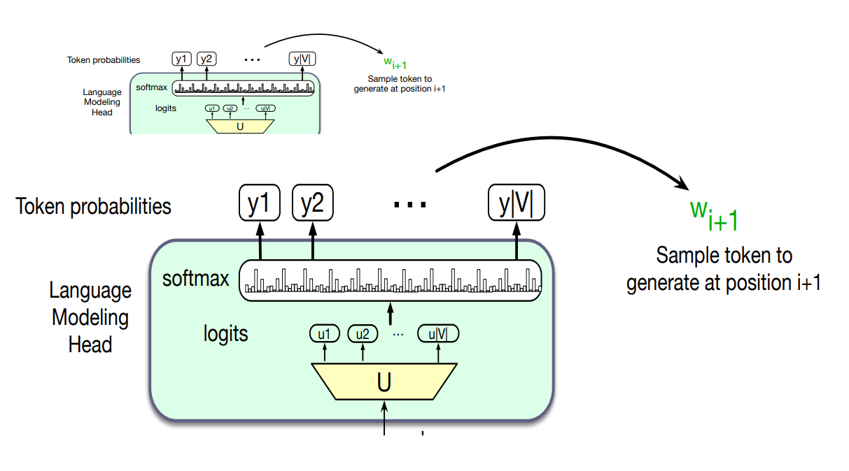
A softmax layer turns the logit into probabilities over the vocabulary , has shape

We can use these probabilities to do things like help assign a probability to a given text, but the most important usage is to generate text, which we do by sampling a word from these probabilities .

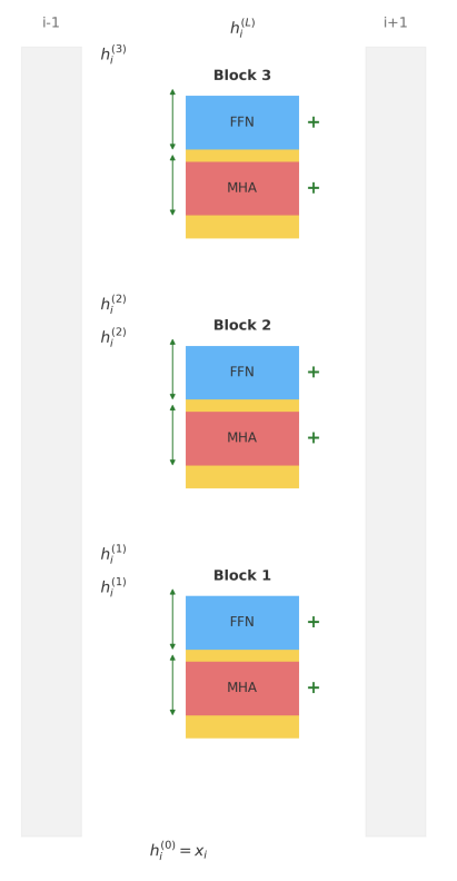
The Final Transformer Model:

The entire stacked architecture for one token :

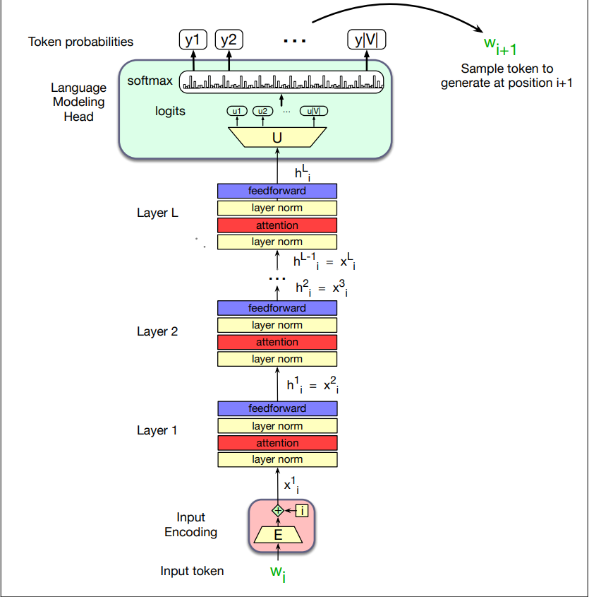
• Note that the input to each transformer layer is the same as the output from the preceding layer .

Training the Transformer §

At each step, given all the preceding words, the final transformer layer produces an output distribution over the entire vocabulary.

During training, the probability assigned to the correct word by the model is used to calculate the cross-entropy loss for each item in the sequence.

Large Language Models are trained with cross-entropy loss also called negative log likelihood loss i.e

The weights in the network are adjusted to minimize the average CE loss over the training sequence via gradient descent.

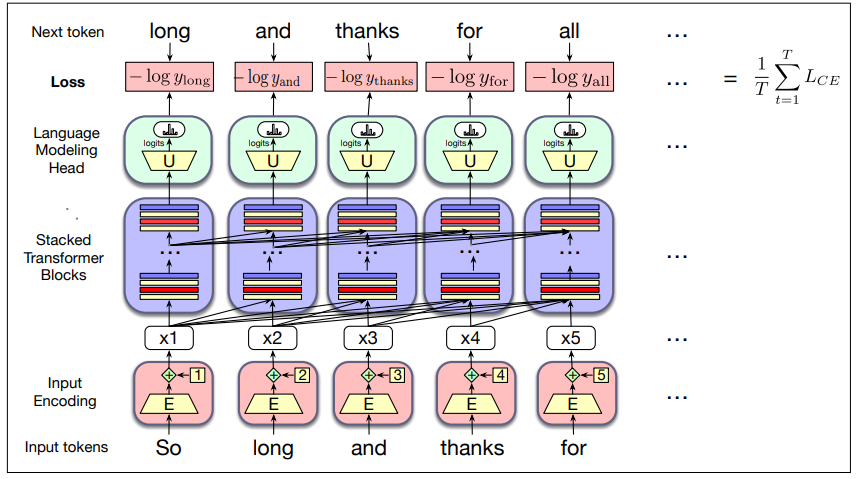
With transformers, each training item can be processed in parallel since the output for each element in the sequence is computed separately (as saw in previous section on parallelization).

Modern LLMs like GPT-4 and LLama 3 have a maximum context window (amount of text they can ingest at once):

• GPT4: 4096 tokens
• Llama 3: 8192 tokens

To maximize training efficiency, we fill this entire window with text for every training example.

If documents are shorter than this, multiple documents are packed into the window with a special end-of-text token between them.

During training, many sequences fit into a single batch:

• Because each sequence is so large (thousands of tokens), the batch size is measured in tokens, not documents
• The batch size for gradient descent is usually quite large (the largest GPT-3 model uses a batch size of 3.2 million tokens)

A transformer used for this kind of unidirectional causal language model is called a decoder only model.

This is because this model constitutes roughly half of the encoder-decoder model for transformers.

Dealing With scale §

Llama 3.1 405B instruct model from Meta has 405 billion parameters ( layers, a model dimensionality of , attention heads) and was trained on 15.6 terabytes of text tokens, using a vocabulary of 128K tokens.

So there is a lot of research on understanding how LLMs scale, and especially how to implement them given limited resources.

Scaling Laws §

Performance of LLM depends on 3 factors:

• model size: the number of parameters not counting embedding
• data size: the amount of training data
• amount of compute used for training

A model can be improved by adding parameters (adding more layers or having wider contexts or both), training more data or by training for more iterations.

The relationships between these factors and performance are known as scaling laws.

Roughly speaking, the performance of a large language model (the loss) scales as a power-law with each of these three properties of model training.

Kaplan et al found the following three relationships for loss as a function of the number of non-embedding parameters , the dataset size and the compute budget for models training with limited parameters, dataset, or computed budget, if in each case the other two properties are held constant:

The number of (non-embedding) parameters can be roughly computed as follows:

• is the input and output dimensionality of the model
• is the self-attention layer size
• is the size of the feedforward layer
• assuming

Thus GPT-3, with layers, a dimensionality of , has billion parameters.

The values depend on the exact transformer architecture, tokenization, and vocabulary size.

Scaling laws can be useful in deciding how to train a model to a particular performance, for example by looking at early in the training curve, or performance with smaller amounts of data, to predict what the loss would be if we were to add more data or increase model size. Other aspects of scaling laws can also tell us how much data we need to add when scaling up a model.

KV Cache §

We saw that the attention vector can be very efficiently computed in parallel for training, via two matrix multiplication:

Unfortunately we can’t do quite the same efficient computation in inference as in training.

At inference time, we iteratively generate the next tokens one at a time.0 For a new token that we have just generated, call it , we need to compute its query, key, and values by multiplying by and respectively.

But it would be a waste of computation time to recompute the key and value vectors for all the prior tokens at prior steps we already computed these key and value vectors.

So instead of recomputing these, whenever we compute the key and value vectors we store them in memory and in the KV cache, and then we can just grab them from the cache when we need them.

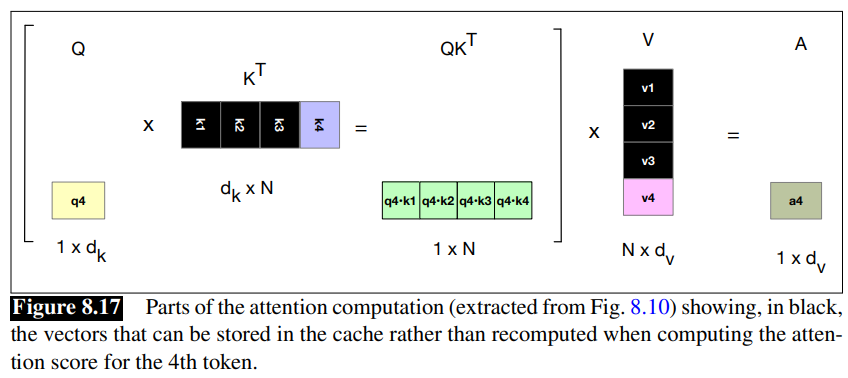
Fig 8.10:

Parameter Efficient Fine Tuning §

It’s very common to take a language model and give it more information about a new domain by finetuing it (continuing to train it to predict upcoming words) on some additional data.

Fine-tuning can be very difficult with very large language models, because there are enormous numbers of parameters to train; each pass of batch gradient descent has to backpropagate through many many huge layers.

There are alternative methods that allow a model to be finetuned without chaing all the parameters. Such methods are called parameter-efficient fine tuning or sometime PEFT.

A subset of parameters to update when finetuning are selected (see feature selection).

Here we describe one such model called LoRA: Low-Rank Adaption

LoRA §

The intuition of LoRA is that transformers have many dense layers which perform matrix multiplication (for example the layers in attention computation).

Instead of updating these layers during finetuning, with LoRA we freeze these layers and instead update a low-rank approximation that has fewer parameters.

Consider a matrix of dimensionality that needs to be updated during finetuning via gradient descent. Normally this matrix would get updates of dimensionality for updating the parameters after graident descent.

In LoRA, we freeze and update instead a low-rank decomposition of . We create two matrices and , where has size and has size . We choose to be quite small: .

During finetuing we update 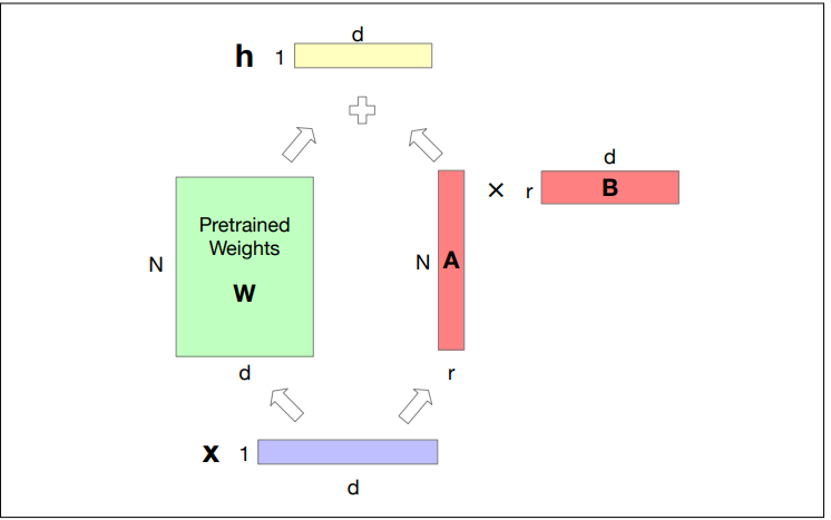and instead of . That is we replace with .

For replacing the forward pass , the new forward pass is instead:

LoRA advantages:

• It dramatically reduces hardware requirements since gradients don’t have to be calculated for most parameters.
• The weights updates can be simply added in to the pretrained weights, since is of the same size as
• It’s possible to build LoRA modules for different domains and just swap them in and out by adding them in or subtractng them from

Interpreting the Transformer §

The subfield of interpretability, sometimes called mechanistic interpretability, focuses on ways to understand mechanistically what is going on inside the transformer.

In-Context Learning and Induction Heads §

As a way of getting a model to do what we want, we can think of prompting as being fundamentally different than pretraining.

Prompting with demonstrations can teach a model to do a new task. The model is learning something about the task from those demonstrations as it processes the prompt. (See [[NLP - Lecture - Large Language Models (LLM)|[NLP] LLM]]).

For example, the further a model gets in a prompt, the better it tends to get at predicting the upcoming tokens. The information in the context is helping give the model more predictive power.

The term in-context learning was first proposed by Brown et al. (202) in their introduction of the GPT3 system, to refer to either of these kinds of learning that language models do from their prompts.

In-context learning means language models learning to do new tasks, better predict tokens, or generally reduce their loss during the forward-pass at inference-time, without any gradient-based updates to the model’s parameters.

We don’t know for sure how in-context learning work.

One hypothesis is based on the idea of induction heads: are the name for a circuit which is a kind of abstract component of a network.

The induction head circuit is part of the attention computation in transformers, discovered by looking at mini-language models with only 1-2 attention heads.

The function of the induction head is to predict repeated sequences.

For example if it see the pattern in an input sequence, it predict that will follow, instantiating the pattern completion rule

It does this by having a prefix matching component of the attention computation that, when looking at the current token , searches back over the context to find a prior instance of . If it finds one, the induction head has a copying mechanism that “copies” the token that followed the earlier , by increasing the probability the will occur next.

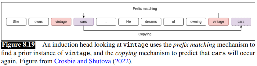
Olsson et al (2022) propose that a generalized fuzzy version of this pattern compeltion rule, implementing a rule like where and (approx means they are semantically similar in some way).

Evidence for their hypothesis come from Crosbie and Shutova (2022) who show that ablating induction heads causes in-context learning performance to decrease. Ablation is a medical term that means removal of something. They find induction heads by first finding attention heads that perform as induction heads on random input sequences, and then zeroing out the output of these heads by setting certain terms of the output matrix to zero.

Logit Lens §

Another useful tool called logit lens (Nostalgebraist, 2020) offers a way to visualize what the internal layer of the transformer might be representing.

The idea is that we take any vector from any layer of the transform and, pretending that it is the prefinal embedding, simply multiply it by the unembedding layer to get logis, and compute a softmax to see the distribution over words that vector might be representing.

Since the network wasn’t trained to make the internal representations function in this way, the logit lens doesn’t always work perfectly.

---