Support Vector Machine (SVM)

See:

• ML1 - Lezione 12 - Kernel Methods and Kuhn and Tucker’s Theorem, SVM prerequisite
• ML1 - Lecture 13-14 - Support Vector Machine, Optimal Hyperplane Problem, Mercer Kernel, Kernel Trick
• ML1 - Lecture 23 - SVM for Regression

It’s an algorithm used both for regression and classification.

An SVM classifier builds a model that assigns new data points to one of the given categories. Thus, it can be viewed as a non-probabilistic binary linear classifier.

• Hyperplane → decision boundary.

• Support Vectors → data points closer to the hyperplane

• Margin → separation gap between data points

• Maximum Margin Hyperplane → The SVM separates data points using a hyperplane with maximum amount of margine.

Support Vector Machine Intuition

The idea behind the kernel methods is to use algorithms that perform implicitly the data in a high dimensional space. For example with an input space of dimension 4 we can go in a space of dimensional 100 and so on.

The Support Vector Machine is the most well known algorithms

It can be summarized into two steps:

1. Project implicitly onto a high-dimensional space by the kernel trick which consists in replacing the innter product between data vectors with a kernel function
2. Apply a linear classification to the projected data

Note that data is projected in a nonlinear way in an higher dimension.

Support Vector Machine Preliminaries Knowledge

Kuhn Tucker Theorem

It is an extension of Lagrange Multipliers for inequality constraints. KTT is used to solve the convex optimization problem i.e., to minimize a convex objective function under certain convex constraints of inequality type, was proposed. There a function must be convex in order to be minimized through inequalities.

Convexness: recall that a set is convex if it contains the interval:

Jensen Inequality: a function is convex if :

Convex Optimization Problem: Let be a linear space and a convex subset of this space . Let and be convex functions.

The convex optimization problems state that we want to minimize under constraints: and for .

Let (x star) be the value that minimizes under constraints and for . Then exists Lagrange multipliers and that are simultaneously not equal to zero and such that the following three conditions hold true:

1. Minimum principle: must minimize the Lagrangian such that
2. Non-negativeness of the conditions: so we cannot have negative values like before
3. Kuhn Tucker Conditions: the product of and called for

If then the previous 3 conditions are sufficient conditions for to be the solution of the optimization problem.

Slater condition: To get , it is sufficient that exists such that the following condition holds: for

Kuhn Tucker Theorem Corollary

If the Slater conditions are satisfied, then one can choose and rewrite the Lagrangian in the form:

Now the Lagrangian is defined as a function of variables and conditions of the Kuhn Tucker theorem are equivalent to the existence of a saddle point () of the lagrangian, i.e:

Optimal Hyperplane Algorithm

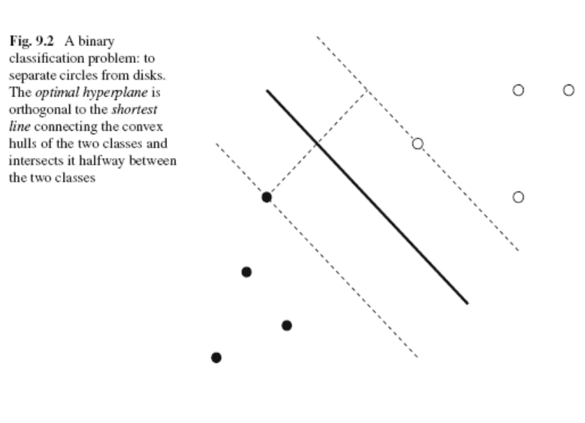For simplicity consider a binary classification problem.

Class of hyperplanes: the general class is defined as: with .

Decision: a signum function is used to decide if a data point appartains to a class or the other. Recall that the signum (sgn) values are -1 if and if .

Optimal Hyperplane: Vapnik and Lener observed that among all hyperplane separating the data exists only one optimal hyperplane that yield the maximum margin of separation between classess:

for all possible value that is the vector of the weights, where

Maximum Margin: distance from a line is computed as: that holds also for an hyperplane. If the point is the closest to the hyperplane it implies that it lies on one of the dotted lines i.e,

Hence: The margin is defined as , so: This implies that margin is inversely proportional to norm of the weights. Hence, maximizing the margin is equivalent to minimizing the norm of weights:

We need to consider an additional constraint: there must be no points between the white and black point that define the margin, expressed through constraint equation:

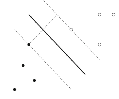So respectively they are either in the upper zone, upper the dotted line or in belove zone belove the zone.

These constraints can be represented into one: where . Now, we want to express this as disequality, so the constraint becomes:

Summary: Optimal Hyperplane Problem

Minimize:

subject to the constraint:

Solution: define a Lagrangian function:

that must be minimizes with respect to weights , bias and maximized with respect to (i.e a saddle point has to be found).

To solve this we use the Kuhn Tucker Theorem introduced before.

The Kuhn-Tucker Theorem want a minus, so the formula for the optimal hyperplane becomes:

Notice: the lagrangian function has lagrangian multiplies, the summation goes from to . So we have as many multipliers as patterns in the dataset.

Support Vectors

Computing the derivative of the Lagrangian respect to the vector we obtain:

So this implies that:

Now we compute the derivative respect to b:

the only things that remains is:

If has a particular value but his respective multiplier is null, then the contribute in the sum of the pattern must be null. This means that the weights depends only by the pattern whose respective multipliers are non-null. These patterns are called support vectors, formaly defined as:

Our problem does not depends on the whole patterns of the dataset but the solution depends only by a particular subset or dataset for by the pattern whose respective Lagrange Multipliers are larger than 0. The other pattern for which the lagrange multiplier are null, in reality, are completely negletted by the algorithm since they don’t influence the value of the weights.

Since we want that:

then the value multiplied by must be null.

So in reality we are not interested by all the points, but only by the two points on the dotted line. 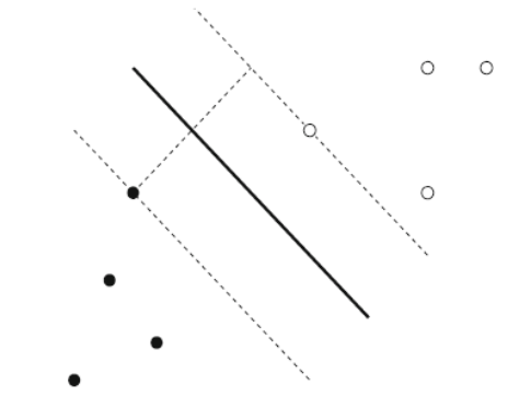These two points are the only points that influences our solution. If you find the support vector, is uniqly determined.

KKT allow us to say that the support vectors, the vectors for which the respective lagrange multipliers is different from zero, lies on the margin, and the other samples of the training set are null.

So, hyperplane is completely determined by the patterns closest to it, the solution should not depend on other patterns of the training set.

We want to get a formula independent from weights: Therefore, the weight can be written as:

Substituting the previous two equations:

in we get:

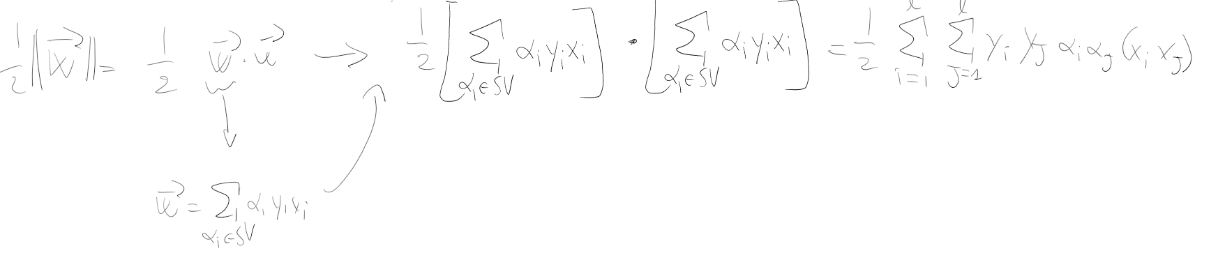Now, consider the term: and substitute as:

(We consider a subset)

Then we obtain:

Then we get the final form by simplfying:

subject to for and

Instead of minimizing , we maximize and we get the final form of the optimization problem.

Note: we did these computations to get a formula independent from .

Hyperplane Decision function

we replace with the expression we computed for before and obtain the formula above.

Now, this is a linear classifier that can solve only linear problems. It cannot solve simple nonlinear problems as XOR.

In order to solve non-linear problem, we need to project data into higher dimension in a nonlinear manner.

Intuition: If the dimension of the new space is high, means that the points are sparse and if the points are sparse, it is more likely that it can be separated by an hyperplane classifier rather than in a smaller space. So we want to project into an higher dimensional space.

So the idea is to substitute this with an appropriate function that we call kernel, Mercel Kernel.

Mercer Kernel

The Mercel Kernel that corresponds to a positive semidefinite function. Let be a nonempty set. A function is called a Mercer Kernel (or positive semidefinite function) if and only if is symmetric () and:

Mercer Kernel Example: Inner Product

An example of mercel kernel is the inner product, defined as: . Replace this expression in the definition and you’ll get:

that is equal to:

Norm is always greater than 0, so the equations holds true and the inner product is a mercer kernel.

The kernel trick consists in this: replacing the inner product with another mercer kernel.

that is always larger than 0, the conseguence is the inner product is a mercer kernel

This is called the kernel trick: replace the inner product with the mercer kernel. At the start of the course we saw the covariance matrix with the proof that is semidefinite positive. And it’s the same, if you compute and G is a kernel, what you get is a matrix that is positive semidefinite.

Mercer Kernel Properties

Cauchy-Swartz Inequality:

Hilbert Space: is a mercer kernel if and only if can be represented as where and is an Hilbert Space.

A mercer kernel must also respect the following properties:

1. Additive property: the sum is again a mercel kernel
2. multiplicity: with note strictly positive, cannot be negative otherwise it doesn’t hold anymore the property saw last lesson
3. - If you take two mercel kernel, the product is again a mercel kernel
4. - If you make the tensorial product of a mercel kernel you get again a mercel kernel.

Where and are two mercer kernels, respectively over and . Also "" is the inner product and "" the tensor product.

Example of Mercer with explicit mapping

• Consider the homogenous kernel of degree 2, i.e:
• Assume the two vectors and are bidimensional vectors
• They can be expressed as: and
• Apply definition to kernel:
• Apply rule of square:

Equation where rule of square is applied is equivalent to:

This is equivalent to using 2 coordinate to make a 6-dimensional space.

Property: this result is generalizable:

Combining Optimal Hyperplane and Mercer Kernel

Implicit mapping If we consider the Gaussian Kernel, the kernel has an implicit mapping since is unknown. Property: Using the gaussian kernel corresponds to project the data with an infinite number of dimensions.

Kernel Trick applied to decision function: Consider the Hyperplane Decision function that i rewrite here for convenience:

Applying the kernel trick means replacing with a kernel in the feature space . So Equation becomes:

Support Vector Machine Construction

Putting together everything from previous section (Support Vector Machine Preliminaries Knowledge) we can construct the SVM.

To construct a SVM, an optimal hyperplane in some Feature Space has to be computed.

The classification of the output assumes only two values

In the Support Vectors section we saw how weight equation can be written as: , but we want to replace the data point with data projected in higher dimension by mercer kernel, that we call .

Problem: is unknown.

Since occur only in scalar products, scalar products can be substituted by an appropriate Mercer kernel , leading to a generalization of the decision function:

This is justified by Mercer Kernel Properties:

Recall the function to minimize defined in Support Vectors. We replace inner product with mercer kernel :

Then we get the final form by simplfying:

subject to constraints:

• for

Slack Variables

In real word problems, there is noise in data (i.e. mislabelled samples), and classes may be partially overlapped. Therefore it is necessary to allow the possibility that some examples can violate the constraint:

A slack variable with is introduced for this. They have the property that they are strictly positive when the respective sample violates the constraint equation, othwerise it is null.

If we introduce these slack variables, the constraints change to this form:

Support Vector Machine objective function

The SVM classifier allows use to control the margin and the number of errors in dataset given by the number of , by the minimization of the objective function.

subject to constraints:

is an hyperparameter called regularization parameter that controls the tradeoff between maximizing the margin and minimizing the classification error.

• Higher penalizes more misclassification, leading to a smaller margin
• Lower allows a larger margin with more tolerance for errors

Notice how with slack variables, we have to minimize that depend not only on the margin but also on the slack variables. Also, SVM is sensitive to outliers because the penalty for misclassification increases linearly with .

The function to minimize is:

subject to constraints:

• with

Sequential Minimal Optimization: That is a quadratic optimization problem, there isn’t an exact solution in numerical analysis and the only way is to use an approximate solution. A greedy approach called sequential minimal optimization consists in optimization using two Lagrange multipliers each time. Since it’s a greedy approach, there is no guarantee that you find an optimal solution.

The number of iterations must be fixed since no convergence is guaranteed.

SVM are binary classifiers: to use it when the number of classes you can use one-versus-rest method or one-versus-one method.

---

Support Vector Machine for Regression

SVM is born as binary classifier, but in the recent years it is more popular for regression, as classification is done with neural networks.

Assume that the output values are

-insensitive loss functon: The idea is to define a -insensitive loss functon that ignores errors that are within a certain distance of true value.

Given a data set and a function the linear 𝜺-insensitive loss function is defined by:

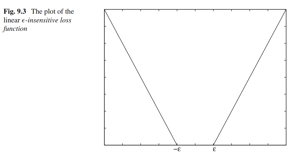
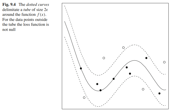Any data point outside this tube, the white circles, has a loss function not null and can be viewed as a training error.

Assumption: assume that is linear,i.e. is an hyperplane that can be described by .

Take the same function to minimize from classification:

Here, we have replaced the term that expresses the number of errors in the classification with the quadratic -insensitive loss.

Now, introducing Slack Variables and constraints we obtain:

Subject to the constraints:

Slack Variables in SVM for regression: and that represents the upper part and below part of the tube. In particular:

• is stricly positive when the respective pattern is such that
• is strictly positive when the respective pattern is such that

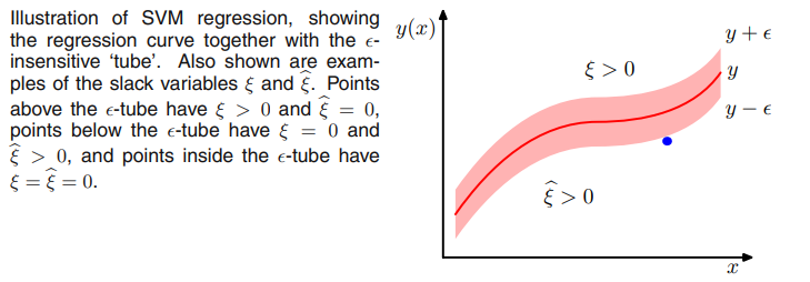
Lagrange Multipliers The usual technique of combining Lagrange variables with Kuhn Tucker Theorem can solve this constrainted optimization problem.

The previous constraints induce two kind of Lagrange multipliers and in the relation: for .

Objective Functions Hence we get the following objective function to maximize

• is the kronecker symbol

subject to constraints:

• both for

The corresponding Kuhn Tucker Conditions are:

• for
• for
• for
• for

Improving the formula: introduce to avoid to have two multipliers to optimize. The objective function formula becomes:

• subject to for

Finally, replace the dot product with the Mercer Kernel:

• subject to for

Regression Estimate: the regression estimates, i.e. the function modelling the data assumes the form:

• where has to be choosen such that:

for any support vector .