AI - Lecture - Solving Problems by Searching - Constraint Satisfaction Problems
In this section we break open the black box by using a factored representation for each state: a set of variables, each of which has a value. A problem is solved when each variable has a value that satisfies all the constraints on the variable.
CSP search algorithms take advantage of the structure of states and use general rather than domain-specific heuristics to enable the solution of complex problems. The main idea is to eliminate large portions of the search space all at once by identifying variable/value combinations that violate the constraints.
Defining Constraint Satisfaction Problems (CSP)
A constraint satisfaction problem consists of three components:
is a set of variables is a domain of possible values , one for each variable is a set of constraints that specify allowable combinations of values.
A domain,
A CSP is a feasibility problem, not necessarily an optimization problem.
Goal: find a value assignment to all variables such that all constraints are satisfied
Optimization vs Satisfaction
Recall that in Search in complex environments we talked about optimization
- Optimization means find the best solution i.e. exactly one solution
- Satisfaction means find any solution
Each constraint
- scope is a tuple of variables that partecipate in the constraint and
- rel is a relation that defines values that those variables can take on.
A relation can be represented as an explicit set of all tuples of values that satisfy the constraint, or as a function that can compute whether a tuple is a member of the relation.
For example, if
or alternatively as:
Assignments and solutions
CSPs deal with assignements of values to variables,
An assignment that does not violate constraints is called a consistent assignement. A complete assignement is one in which every variable is assigned a value, and a solution to a CSP is a consistent, complete assignement.
A partial assignement leaves some variables unassigned, and a partial solution is a partial assignment that is consistent.
Solving a CSP is a NP-complete problem in general, altough here are important subclasses of CSPs that can be solved very efficiently.
Hards and soft constraints:
- hard constraints must be satisfied by every valid solution. They define the set of feasible assignements. For example in Sudoku, each number must satisfy row, column and subgrid rules
- Soft constraints express preferences. May be violated but violations incur a cost or reduce a preference score used to rank feasible solutions.
Example problem - Exam scheduling
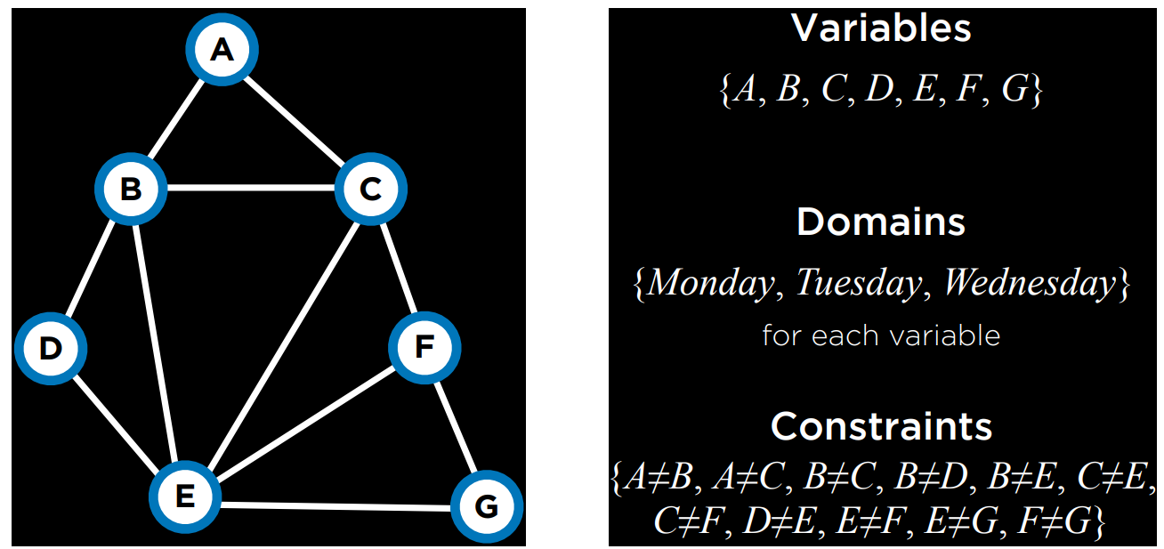
- Variables: one variable for each exam - A,B,C,D,E,F,G
- Domain: available exam days - Monday, Tuseday, Wednesday for each variables
- Constraint: connected exams cannot be assigned the same day
- For every edge
, we impose - A valid schedule is a complete, conflict-free assignment
Constraints can be expressed as:
🧩 Example Problem - Map Coloring of Australia
We are given the task of coloring each region either red, green, or blue in such a way that no two neighboring regions have the same color.
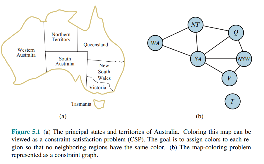
To formulate this as a CSP, we define the variables to be the regions:
The domain of every variable is set
The constraints require neighboring regions to have distinct colors. Now since there are nine places where regions border, there are nine constraints:
In this case,
There are many possible solutions to this problem, such as:
It can be helpful to visualize a CSP as a constraint graph, where the nodes corresponds to variables of the problem and an edge connects any two variables that partecipate in a constraint.
Atomic state-space search vs CSP:
- For example if we consider this problem without constraints, we would have an atomic state-space searcher that should consider
assignements. - With a CSP, and choosen an initial state i.e.
then we can conclude that none of the five neighboring variables can take on the value blue - With constraints our problem has only
assignements, reducing by 87% the complexity
With CSP once we find that a partial assignement violates a constraint, we can immediately discard further refinements of the partial assignment.
Furthermore, we can see why the assignment is not a solution—we see which variables violate a constraint—so we can focus attention on the variables that matter.
As a result, many problems that are intractable for atomic state-space search can be solved quickly when formulated as a CSP.
The 8-Queens problem can also be viewed as a finite-domain CSP.
The best-known category of continuous-domain CSPs is that of linear programming problems, where constraints must be linear equalities or inequalities.
In addition to examining the types of variables that can appear in CSPs, it is useful to look at the types of constraints. The simplest type is the unary constraint, which restricts the value of a single variable. A binary constraint relates two variables. A binary CSP is one with only unary and binary constraints.
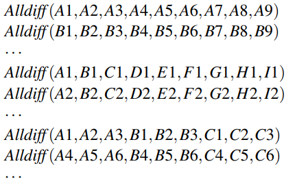
A constraint involving an arbitrary number of variables is called a global constraint. One of the most common global constraints is called Alldiff, which says that all the variables involved in constraint must have different values. For example in Sudoku problems, all variables in a row, column or 3x3 box must satisfy the Alldiff constraint.
Another example is provided by cryptarithmetic puzzles. Each letter in a cryptarithmetic puzzle represents a different digit. The addition constraints on the four columns of the puzzle can be written as the following n-ary constraints:
,
where
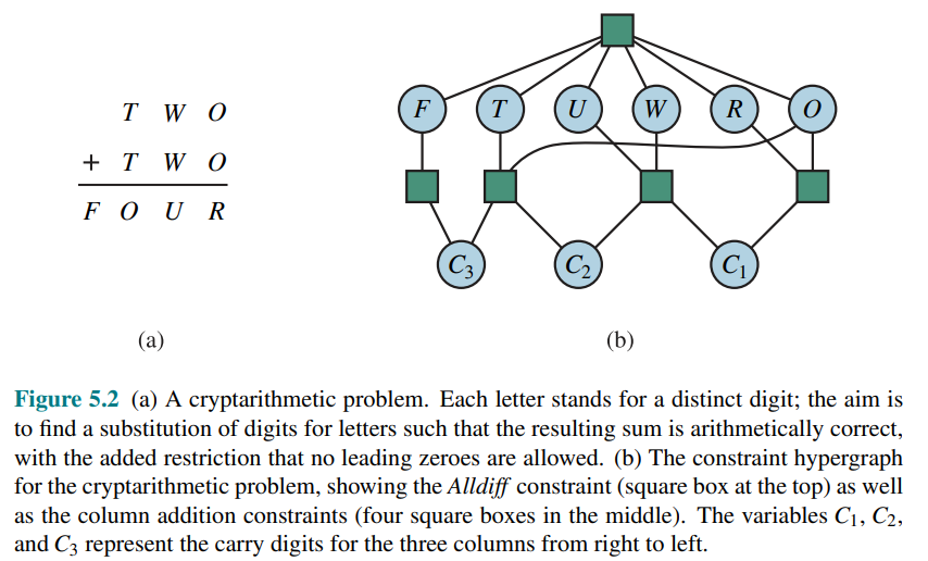
Dual graph: another way to convert an n-ary CSP to a binary one is the dual graph transformation: create a new graph in which there will be one variable for each constraint in the original graph, and one binary constraint for each pair of constraints in the original graph that share variables.
Preference Constraints: Many real-world CSPs include preference constraints indicating which solutions are preferred. For example, in a university class-scheduling problem there are absolute constraints that no professor can teach two classes at the same time. But we also may allow preference constraints: Prof. R might prefer teaching in the morning, whereas Prof. N prefers teaching in the afternoon.
Preference constraints can often be encoded as costs on individual variable assignments—for example, assigning an afternoon slot for Prof. R costs 2 points against the overall objective function, whereas a morning slot costs 1. With this formulation, CSPs with preferences can be solved with optimization search methods, either path-based or local. We call such a problem a constrained optimization problem, or COP. Linear programs are one class of COPs.
Question: Is Support Vector Machine a kind of CSP?
A Support Vector Machine (SVM) is not strictly a Constraint Satisfaction Problem (CSP), but rather a Constraint Optimization Problem (COP). While a CSP seeks any assignment that satisfies all constraints (feasibility), an SVM seeks the assignment that maximizes the margin (optimality).
In the SVM framework, the variables are the weights (
) and bias ( ), and the constraints are the classification requirements for training data points. The objective function—minimizing —distinguishes it from a standard feasibility-only CSP. For more details on the SVM formulation, see Support Vector Machine (SVM). Mathematically, SVM is a Quadratic Programming (QP) problem. This aligns it with Linear Programming (LP), which your notes identify as a key class of continuous-domain CSPs, but adds a quadratic objective for the maximum margin.
In summary, SVM uses the same “factored representation” of states (variables and constraints) as CSPs but is solved using convex optimization techniques like Lagrange Multipliers rather than search-based algorithms.
Constraint Propagation - Inference in CSPs
While an atomic state-space algorithm makes progress only by expanding a node to visit the successor, CSP algorithms can make choices. They can generate successors by choosing a new variable assignment, or it can do a specific type of inference called constraint propagation.
Constraint propagation consists in using the constraints to reduce the number of legal values for a variable, which in turn can reduce the legal values for another variable, and so on.
The key idea is local consistency: the process of enforcing local consistency in each part of the graph causes inconsistent values to be eliminated throughout the graph.
There are different types of local consistency, which we now cover in turn.
Node Consistency
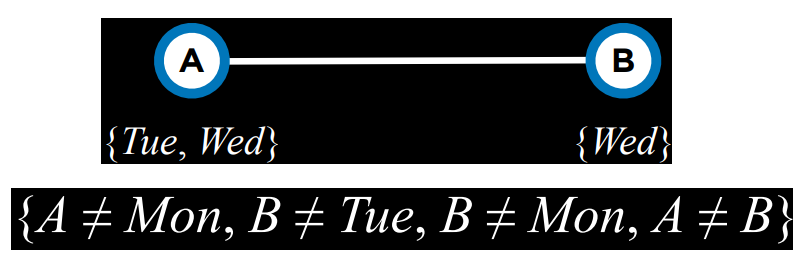
The first one is Node Consistency. It concerns unary constraints, a variable is node-consistent if every value in its domain satisfies all unary constraints on that variable. Enforcing node consistency means removing values that violate unary constraints.

- In the previous image: we have to remove Monday from A’s domain.
- Iterate and apply also to other variables and you’ll end up with the following:
Arc consistency
A variable in a CSP is arc-consistent (i.e. edge-consistent) if every value in its domain satisfies the variable’s binary constraints.
More formally:
A graph is arc-consistent if every variable is arc-consistent with every other variable.
An example of arc-consistency is for the constraint
To make X arc-consistent with respect to Y, we reduce X’s domain to
On the other hand, arc consistency can do nothing for the Australia map-coloring problem. For example with the inequality constraint on (SA,WA):
No matter what value you choose for SA, there is a valid value for the other variable. So applying arc consistency has no effect on the domains of either variable.
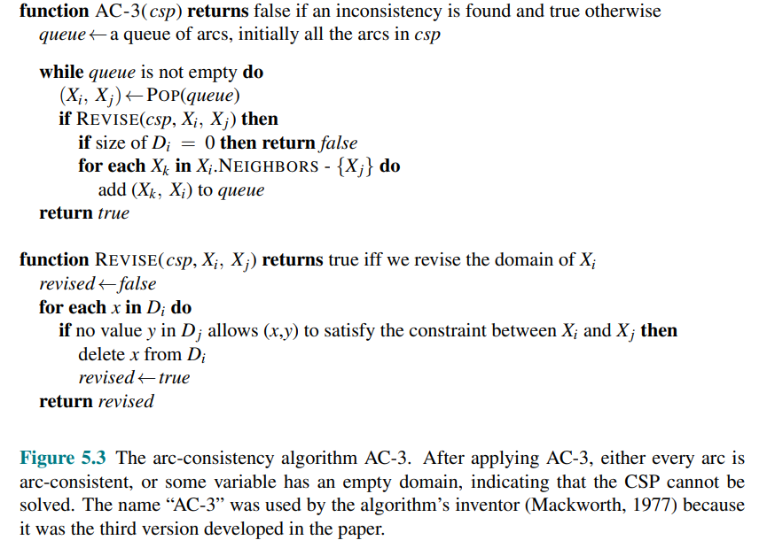
The most popular algorithm for enforcing arc consistency is called AC-3. To make every variable arc-consistent, the AC-3 algorithm maintains a queue of arcs to consider. Initially, the queue contains all the arcs in the CSP. (Each binary constraint becomes two arcs, one in each direction.) AC-3 then pops off an arbitrary arc
Sudoku
A Sudoku board consists of 81 squares, some of which are initially filled with digits from 1 to 9.
The puzzle is to fill in all the remaining squares such that no digit appears twice in any row, column, or 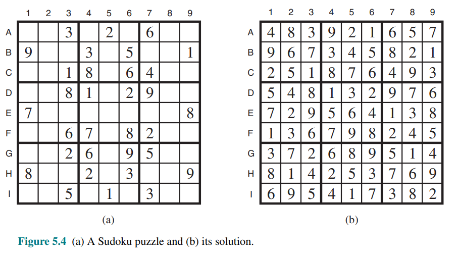
The Sudoku have the property that they have exactly one solution. Although some can be tricky to solve by hand, taking tens of minutes, a CSP solver can handle thousands of puzzles per second.
A Sudoku puzzle can be considered a CSP with 81 variables, one for each square.
There are 27 different Alldiff constraints, one for each unit:
Let’s see how far we can go with arc consistency.
If we consider E6, from the constraints in the box we can remove 1,2,7 and 8 from
Inference continues along these lines, and eventually, AC-3 can solve the entire puzzle—all the variables have their domains reduced to a single value, as shown in Figure 5.4.
AC-3 works only for the easiest Sudoku puzzles. Slightly harder ones can be solved by PC-2, but at a greater computational cost: there are 255.960 different path constraints to consider in a Sudoku puzzle. To solve the hardest puzzles and to make efficient progress, we will have to be more clever.
Backtracking Search for CSPs
Sometimes we can finish the constraint propagation process and still have variables with multiple possible values. In that case we have to search for a solution. In this section we cover backtracking search algorithms that work on partial assignments.
Intuition: If you make a choice (assigning a value to a variable) and that choice violates a constraint, Backtracking lets you realize it immediately, “retrace your steps” (backtrack), and try another path.
CSP as search problem:
- State: a partial assignment of values to variables
- Initial state: the empty assignment
- Action: assign a value to one unassigned variable
- Transition model: extend the current partial assignment
- Goal test: the assignment is complete and consistent
- Path cost: usually not relevant in classical CSPs, since the goal is to find any feasible solution
- Therefore, CSP solving is a search over partial assignments
Commutativity: Consider how a standard depth-limited search apply to CSPs.
- A state would be a partial assignment, and an action would extend the assignment, adding, say, NSW = red or SA = blue for the Australia map-coloring problem.
- For a CSP with n variables of domain size d we would end up with a search tree where all the complete assignments (and thus all the solutions) are leaf nodes at depth n.
- But notice that the branching factor at the top level would be
because any of values can be assigned to any of variables. - At the next level, the branching factor is
and so on for levels. - The tree has
leaves, even though there are only possible complete assignments! - We can get back that factor of
by considering that the order of application of any given set of action does not matter in this case. In CSPs, it makes no difference if we first assign NSW = red and then SA = blue, or the other way around - Therefore, we need only consider a single variable at each node in the search tree.
Backtracking Algorithm
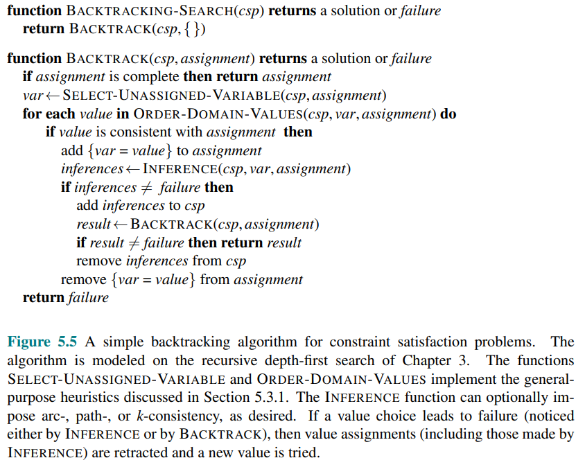
Backtracking search can be improved using domain-independent heuristics that take advantage of the factored representation of CSP.
SELECT-UNASSIGNED-VARIABLE and ORDER-DOMAIN-VALUES implement the general purpose heuristcs that will be discussed in the following sections.
🧠 Mnemonic cheat sheet
- The Problem (Standard Search Tree):
- Branching Factor: Starts at
, drops to at next level, etc. - Total Leaves:
(Unnecessary overhead due to variable ordering permutations). - Reality check: There are only
possible complete assignments. - The Solution (Commutativity):
- Core property: CSPs are commutative
the order of variable assignments does not matter (e.g., is identical to ). - Pruning the
: We only consider a single pre-chosen variable at each node in the search tree. - New Branching Factor: Drops from
to just . Total leaves successfully reduced to . - Backtracking Algorithm:
- A modified Depth-First Search (DFS) for partial assignments that checks constraints as it goes and backtracks immediately upon failure.
- Boosted by two key general-purpose heuristics:
SELECT-UNASSIGNED-VARIABLE(which variable to pick next) andORDER-DOMAIN-VALUES(which value to try first).
Variable ordering and Value ordering
Intuition: these are heuristics (see heuristic search strategies), they tell you where to start (variable ordering) and what to try first (value ordering)
- For variable ordering we want to fail as soon as possible to avoid useless subtrees
- Once you find a variable (i.e. the region on the map), you have to decide which value to try first (i.e. green, red, blue…). Here we want to make the problema easier for the future
Consider the line:
var <- SELECT-UNASSIGNED-VARIABLE (csp, assignement)
The simplest strategy for SELECT-UNASSIGNED-VARIABLE is static ordering i.e. choose the variable in ordering
Minimum-remaining-values (MRV) heuristic: choosing the variable with the fewest “legal” values. It picks a variable that is most likely to cause a failure soon, thereby pruning the search tree.
If some variable X has no legal values left, the MRV heuristic will select X and failure will be detected immediately—avoiding pointless searches through other variables.
However this doesn’t help in choosing the first region to color in Australia. Another heuristic is the
Degree heuristic: it attempts to reduce the branching factor on future choices by selecting the variable that is involved in the largest number of constraints on other unassigned variables.
Typical strategy:
- apply MRV first,
- then use the degree heuristic to break ties
Once a variable has been selected, the algorithm must decide on the order in which to examine its values. The least-constraining value heuristic is effective for this. It prefers the value that rules out the fewest choices for the neighboring variables in the constraint graph.
For example suppose that we have generated the partial assignement with WA=red and NT=green and that our next choice is for Q. Blue would be a bad choice because it eliminates the last legal value left for Q’s neighbor, SA. The least-constraining value heuristic therefore prefers red to blue. In general, the heuristic is trying to leave the maximum flexibility for subsequent variable assignments. LCV prefers the value that makes the future problem easiest, not the current step easiest
Mnemonic cheat sheet - heuristics for variable and value ordering
Variable Ordering: which region to try first, second, third…?
- MRV: choose the variable with less remaining options.
- Degree Heuristic: break ties created by MRV by choosing the variable involved with the largest number of constraint on unassigned values
Value ordering: which color to try to assign first?
- Less-Constraining Value (LCV): Choose the value that constrains the neighbors the least.
- Be a good neighbor and leave your neighbors with the most flexibility possible.
🧩Interleaving search and inference
Inference can be even more powerful during the course of a search: every time we make a choice of a value for a variable, we have a brand-new opportunity to infer new domain reductions on the neighboring variables.
One of the simplest forms of inference is called forward checking. Whenever a variable X is assigned, the forward-checking process establishes arc consistency for it: for each unassigned variable Y that is connected to X by a constraint, delete from Y’s domain any value that is inconsistent with the value chosen for X.
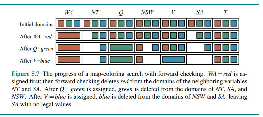 Hence, forward checking has detected that this partial assignment is inconsistent with the constraints of the problem, and the algorithm backtracks immediately.
The problem is that forward checking does not detect all the inconsistencies. For example in Figure 5.7, at row After Q=green, we’ve made WA and Q arc-consistent, but we’ve left both NT and SA with blue as their only possible value, which is an inconsistency, since they are neighbors.
The algorithm called Maintaining Arc Consistency (MAC) checks this kind of inconsistencies. After a variable INFERENCE procedure calls AC-3, but instead of a queue of all arcs in the CSP, we start with only the arcs
From there, AC-3 does constraint propagation in the usual way, and if any variable has its domain reduced to the empty set, the call to AC-3 fails and we know to backtrack immediately.
MAC recursively propagate constraints when changes are made to the domains of variables.