---

AI - Lecture - Solving Problems by Searching - Heuristic Search Strategies and Heuristic Functions

• Source: Book Artificial Intelligence A Modern Approach 4 edition global edition - Russel - Chapter 3

Recall:

• Uninformed Search Strategies in particular, how to measure problem-solving performance

Informed (Heuristic) Search Strategies

Uninformed search strategies are slow and using an heuristic can help to find solutions more efficiently. In informed search strategies, an agent can estimate the cost from the current state to the goal state using an heuristic function.

Heuristic function: denoted as is defined as the estimated cost of the cheapest path from the state at node n to a goal state.

• Example: in route-finding problems, we can estimate the distance from the current state to a goal by computing the straight-line distance on the map between the two points.

Heuristic Function intuition

says how much it take to reach the goal state.

Example, in route-finding problems is distance remaining estimate.

If you are in one city and want to reach another, you can ignore the actual road network and use the straight-line distance between the two points. This distance is not the real travel distance on roads, but it provides a good estimate of how far apart the two locations are.

Greedy best-first search

Expands first the node with the lowest value, the node that appears to be the closest to the goal. The evaluation function in this case becomes .

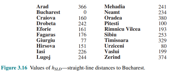
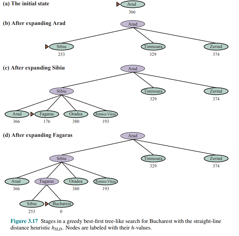
Applied to the route-finding problem in Romania, we compute first the straight-line distance heuristic called ; if the goal is Bucharest, we need to know the straight-line distances to Bucharest.

For this kind of problem, the greedy best-first search find the solution without even expanding a node that is not on the solution path.

Greedy best-first graph search is complete in finite state spaces, but not in infinite ones.

The worst-case time and space complexity is . However with a good heuristic function the complexity can be reduced substantially, on certain problems reaching .

A* Search

The most common informed search algorithm is A star search, that uses the evaluation function:

• is the path cost from the initial state to node n
• is the estimated cost of the shortest path from n to a goal state, so we have:

Consider following figure:

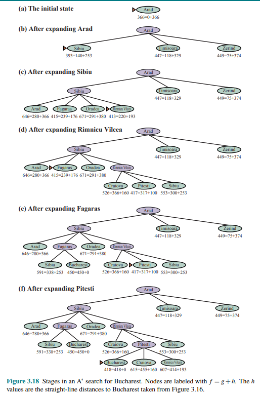
The values of are computed from the action costs, and the values of (straight line distance) are computed as in the Greedy best-first search section.

Notice that at step (e), Bucharest appears on the frontier with a cost of 450, however the algorithm does not select it because there is a possibility that going through Pitesti, whose cost is as low as 417, a better solution would be find. In fact, at step (f), After Pitesti Bucharest is selected as the lowest at , so it is selected and detected as the optimal solution.

graph LR

Greedy("Greedy best-first search")-->GreedyFunction("$$f(n)=h(n)$$")
Astar("$$A^*$$")-->AstarFunction("$$f(n)=g(n)+h(n)$$")

Admissible Heuristic

• search is complete assuming all action costs are and the state space either has a solution or is finite.
• A key property is admissibility, an admissible heuristic is one that never overestimates the cost to reach a goal (an admissible heurstic is therefore optimistic).
• With an admissible heuristic, is cost-optimal

In short: is complete with positive step cost, and with an admissible (optimistic) heuristic that is guaranteed to return the optimal path.

Admissible heuristic example + clarification

In the 8-puzzle, a good heuristic is the number of misplaced tiles. It is admissible since each misplaced tile must be moved atleast once, so the estimate never exceeds the true number of moves required. For example, if at state , and the true minimal cost to solve the puzzle from is for example 6 moves, then then this is an admissible heuristic

Admissibility is about the accuracy of the estimate at each individual state, not about its monotonicity along a path. The heuristic evaluates each state independently. It is allowed to go up or down during search; what matters is only that it never gives a value larger than the real remaining cost to the goal.

Consider this eight puzzle:

1 2 3
4 5 6
7 _ 8

Two possible moves: either slide 7 or 8. If we slide 7, then the number of misplacing tiles i 2, so where is the number of true optimal cost to goal. If we slide 8, then we reach the goal since , and there are no more moves so . As you can see it never overestimated it.

Proof by contradiction that is optimal

• Suppose the optimal path has cost , but the algorithm returns a path with cost
• Then there must be some node n which is on the optimal path and is unexpanded (because if all the nodes on the n the optimal path had been expanded, then we would have returned that optimal solution)

Let be the cost of the optimal path from the start to and let be the cost of the optimal path from to the nearest goal, we have:

• (otherwise n would have been expanded)
• by definition
• because we said that n is on the optimal path
• If we consider admissibiliy then then we can write:
• Then because by definition

However, the first and the last lines from a contradiction, so the supposition that the algorithm could return a suboptimal path must be wrong: it must be that returns only cost-optimal paths.

Consistent Heuristic

Another slightly stronger property is called consistency. An heuristic is consistent if, for every node n and every successor of n generated by an action a we have:

This is a form of the triangle inequality i.e a side of a triangle cannot be longer than the sum of the other two sides.

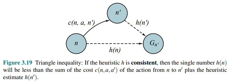
• The direct estimate of going from to a goal can never exceed the cost of going from to plus estimate from to the goal.

Every consistent heuristic is admissible but not viceversa, so is cost-optimal.

In addition, with a consistent heuristic, the first time we reach a state it will be on an optimal path, so we never have to re-add a state to the frontier, and never have to change an entry in reached. With an inconsistent heuristic, we may end up with multiple paths reaching the same state, and if each new path has a lower path cost than the previous one, then we will end up with multiple nodes for that state in the frontier, costing us both time and space.

These complications have led many implementers to avoid inconsistent heuristics, but Felner et al. (2011) argues that the worst effects rarely happen in practice, and one shouldn’t be afraid of inconsistent heuristics.

Search Contours

A useful way to visualize a search is to draw contours in the state space, just like the contours in a topographic map.

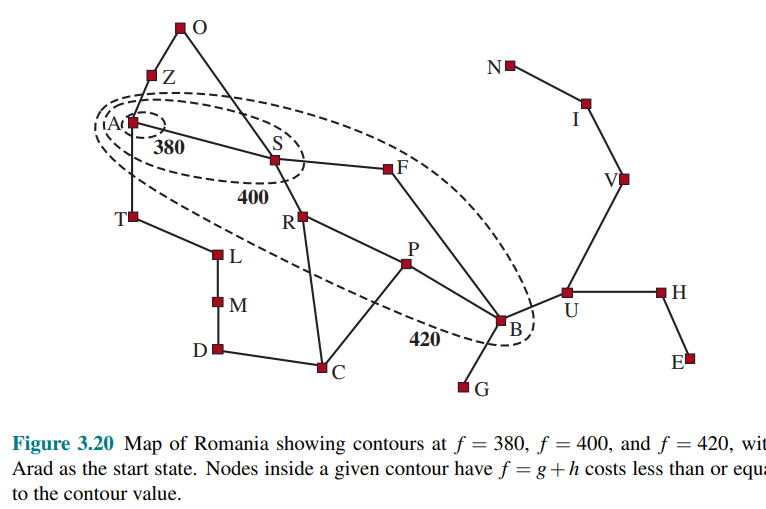
In the contour labeled 400 in the figure, all the nodes have and so on.

• In a search, the algorithm expands the frontier node of lowest f-cost, adding nodes in the concentric bands of increasing -cost
• With uniform cost-search, we also have contours but of -cost, not The contours with uniform-cost search will be “circular” around the start state, spreading out equally in all directions with no preference towrds the goal
• A good heuristic will make the search stretch toward a goal state and become more narrowly focues around a optimal path
• The costs are monotonic: the path always increases as you go along a path, because action costs are always positive. Therefore you get concentric contour lines that don’t cross each other.
• However it is not obvious if cost will monotonically increase.

A* properties: surely expanded nodes and optimally efficient

If is the cost of the optimal solution path, we can say that:

• Surely expanded Nodes: expands all nodes that can be reached from the initial state on a path where every node on the path has .
• if might expand some of the nodes right on the “goal contour if it expands no nodes with .

is complete unless there are infinitely many nodes with f ≤ f(goal). is optimal if the heuristic is admissible

is optimally efficient in the sense that expand fewer nodes with respect to other optimal algorithms using the same heuristic

has exponential worst-case time and space complexity, however, it is much more efficient (generates a much smaller number of nodes) than other uninformed and informed search strategies.

Memorization tips

Search space can be visualized as contours (levels) like a topographic map.

• and in particular expands in bands around the start toward the goal. is monotonic toward the goal
• For the greedy best-first search these are circular
• A good heuristic makes contours “stretch” toward the goal.

The then has this property:

• With a consistent heuristic, is optimally efficient since no other optimal algorithm using the same heuristic can expand fewer nodes.

Pruning

is efficient because it prunes away search tree nodes that are not necessary for finding an optimal solution. The concept of “pruning” i.e eliminating possibilities from consideration without having to examine them, is important for many areas of AI.

Problems of A star search

isnt necessarily the answer to all our searching needs. The catch is that for many problems, the number of nodes expanded can be exponential in the length of the solution.

For example: consider a version of the vacuum world with a super-powerful vacuum that can clean up any one square at a cost of 1 unit, without even having to visit the square. In that scenario, squares can be cleaned in any order.

With initially dirt squares, there are states where some subset has been cleaned; all of those states are on an optimal solution path, and hence satisfy , so all of them would be visited by .

graph LR
    AStar[A*]
    Function[f=g+h]
    Admissible[Admissible]
    Consistent[Consistent]
    Contours[Contours]
    Stretch[Stretch toward goal]
    Efficient[Efficient]
    Pruning[Pruning]
    Complexity[Exponential complexity]
    CostOptimal["Cost Optimal"]
    OptimalPath["Optimal Path"]

    AStar --> Function
    Function --> Admissible --> CostOptimal
    Function --> Consistent --> OptimalPath
    AStar --> Contours
    Pruning --> Efficient
    AStar --> Pruning
    AStar --> Complexity
    Contours-->Stretch

Satisficing Search: Inadmissible heuristics and weighted A*

Satisficing Solution: search expands a lot of nodes. We can explore fewer nodes (taking less time and space) if we are willing to accept solutions that are suboptimal but are “good enough” what we call satisficing solutions.

If we allows search to use an inadmissible heuristic i.e that can overstimate, then we risk missing the optimal solution, but it can be potentially more accurate, reducing the number of nodes expanded.

For example, road engineers know the concept of detour index, which multiplier applied to the straight-line distance to account for typical curvature of a road. A detour index of 1.3 means that if two cities are 10 miles apart in straight-line distance, a good estimate of the best path between them is 13 miles. For most localities, the detour index ranges between 1.2 and 1.6.

This can be applied to any problem, not just ones involving roads, with an approach called weighted A star search, where we weight the heuristic value more heaviliy, giving us the evaluation function:

Figure 3.21 shows a search problem on a grid world.

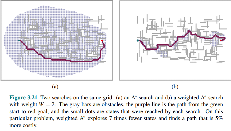
• In (a) it finds the optimal solution, but has to explore a large portion of the state space to find it
• In (b), a weighted search finds a solution that is slightly costlier, but the search time is much faster.

If the optimal solution costs , a weighted will cost , but in practice we get results much closer to than .

• search: ()
• Uniform-cost search: , ()
• Greedy best-first search: ,
• Weighted search:

You could call weighted “somewhat-greedy search”: like greedy best-first search, it focuses the search towards a goal; on the other hand, it won’t ignore the path cost completely, and will suspend a path that is making little progress at great cost.

Greedy vs A star

the most important difference between greedy and A star is that the greedy best-first search ignores the path cost

Suboptimal search algorithms

There are a variety of suboptimal search algorithms, which can be characterized by the criteria for what counts as “good enough”:

• bounded suboptimal search: we look for a solution that is guaranteed to be within constant factor of the optimal cost
• bounded-cost search: we look for a solution whose cost is less than some constant
• unbounded-cost search: we accept a solution of any cost, as long as we can find it quickly

One example is the speedy search which is a variant of the greedy best-first search that uses as a heuristic the estimated number of action required to reach a goal, regardless of the cost of those actions.

🧩 Memory-bounded search

One main issue of is its use of memory.

Memory use is split between the frontier and the reached states.

Using the “best-first search” implementation (see Best-First Search), a state that is on the frontier is stored in two places: as a node in the frontier and as an entry in the table of reached states. One possible improvement is to keep a state in only one of the two places, saving a bit of space at the cost of complicating the algorithm. Another is to keep reference counts of the number of time a state has been reached, and remove it from the reached table when there are no more ways to reach the state.

Now let’s consider new algorithms designed to conserve memory usage.

Beam Search

Beam search limits the size of the frontier, keeping only the nodes with the best -scores, discarding any other expanded nodes. This makes the search incomplete and suboptimal, but we can choose to make good use of availability memory, and the algorithm executes fast because it expands fewer nodes.

For many problems it can find good near-optimal solutions.

Another variant consider keeping every node whose -score is within of the best -score. That way, when there are a few strong-scoring nodes only a few will be kept, but if there are no strong nodes then more will be kept until a strong one emerges.

Iterative-deepening search ()

It is similar to Iterative deepening search.

Gives the benefit of without the requirement to keep all reached states in memory, at a cost of visiting some states multiple times.

It is a very important and commonly used algorithm for problems that do not fit in memory.

How IDA star works

• Start with an initial limit f-cutoff=
• Run a DFS algorithm where you expand only a node with . If a node > you cut it and save his
• At the end of the iteration, update the cutoff variable with the minimum value of between the cut nodes
• Repeat until you find the goal

In the cutoff is the -cost (); at each iteration, the cutoff value is the smallest -cost of any node that exceeded the cutoff on the previous iteration.

For problems like the 8-puzzle where each path’s -cost is an integer, this works very well, resulting in steady progress towards the goal each iteration.

For a problem where every node has a different -cost, each new contour might contain only one new node, and the number of iterations could be equal to the number of states.

Recursive best-first search (RBFS)

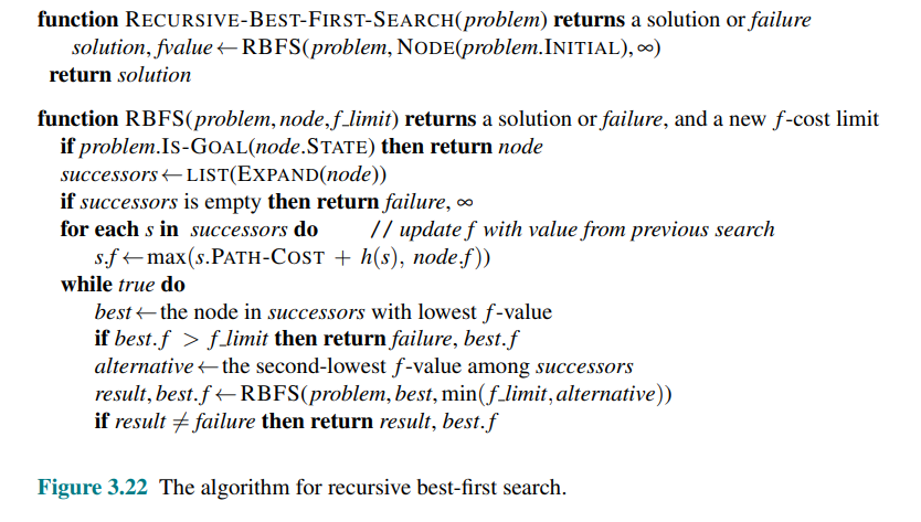
RBFS attempts to mimic the operation of standard best-first search, but using only linear space.

RBFS resembles a recursive depth-first search, but rather than continuing indefinitely down the current path, it uses the limit variable to keep track of the -value of the best alternative path available from any ancestor of the current node. If the current node exceeds this limit, the recursion unwinds back to the alternative path.

Intuition:

• When you are at a node n, RBFS does not only consider that node, but also the best alternative among its siblings (i.e., other already generated paths).
• This value is passed as: the best available alternative outside the current branch.

As the recursion unwinds, RBFS replaces the -value of each node along the path with a backed-up value — the best -value of its children. In this way, RBFS remembers the -value of the best leaf in the forgotten subtree and can therefore decide whether it’s worth reexpanding the subtree at some later time.

Intuition:

• even if a branch is temporarily abandoned, it is not forgotten; it is represented by the best f-value discovered within its subtree.

In the following figure the algorithm is shown:

And in the following one, stages of a RBFS search for the shortest route to Bucharest.

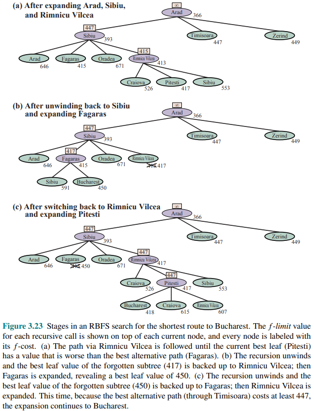
RBFS is optimal if the heuristic function is admissible.

Its space complexity is linear in the depth of the deepest optimal solution, but its time complexity is rather difficult to characterize: it depends both on the accuracy of the heuristic function and on how often the best path changes as nodes are expanded. It expands nodes in order of increasing -score, even if is nonmonotonic.

Memory-bounded A star and SMA star

and RBFS suffer from using too little memory, as conseguence they forget most of what they have done and may end up re-exploring the same states many times over.

To solve this, two algorithms variante are MA star (memory-bounded and SMA star (simplified MA). We explain the simplified version there.

proceeds just like , expanding the best leaf until memory is fully. At this point, it cannot add a new node to the search tree without dropping an old one. Well, always drop the worst leaf node i.e the one with the highest f-value. Then, like RBFS, backs up the value of the forgotten node to its parent.

With this information regenerates the subtree only when all other paths have been shown to look worse than the path it has forgotten. In other words, if all the descendants of the node n are forgotten, we will not know which way to go from n but we still have an idea how worthwhile it is to go anywhere from n.

Clarification on SMA*

How it works:

1. It starts like i.e. expand the node with lowest , until it fills the memory
2. When the memory is fully, it must delete a node: the worst leaf i.e. the leaf with the highest value.
3. Before deleting it, this value is “backed-up” in the father node.
4. In this way SMA know that from that subtree, the best resulting value was , so it know the potential of that part of the space and can more intelligenly choose to ignore it or take it

is complete if there is any reachable solution, that is if , the depth of the shallowest goal node, is less than the memory size (expressed in nodes). It is optimal if any optimal solution is reachable; otherwise, it returns the best reachable solution

Limitations of : On very hard problems, however, it will often be the case that SMA∗ is forced to switch back and forth continually among many candidate solution paths, only a small subset of which can fit in memory. (This resembles the problem of thrashing in disk paging systems.). The extra time required for repeated regeneration of the same nodes means that the problems that would be practically solvable by given unlimited memory, become intractable for . That is, to say, memory limitations can make a problem intractable from the point of view of computation time.

🧩 Bidirectional heuristic search

With bidirectional search, it turns out that it is not individual nodes but rather pairs of nodes (one from each frontier) that can be proved to be surely expanded.

We use:

• for nodes going in the forward direction (with the initial state as root) and
• for nodes in the backward direction (with a goal state as root).

They solve the same problem but different notation is required because different evaluation functions are required for example due to different heurstics depending on whether you are striving for the goal or for the initial state. We assume admissible herustics.

Consider a forward path from the initial state to a node and backward path from the goal to a node . The lower bound on the cost of a solution that follows the path from the initial state to , then somehow gets to , then follows the path to the goal as:

In other words, the cost of such a path must be at least as large as the sum of the path costs of the two parts (because the remaining connection between them must have nonnegative cost), and the cost must also be at least as much as the estimated cost of either part (because the heuristic estimates are optimistic).

For any pair of nodes with less than the optimal cost , we must expand either or because the path that goes through both of them is a potential optimal solution. The difficulty is we don’t know for sure which node is the best to expand, and therefore no bidirectional search algorithm can be guaranteed to be optimally eficient.

The evaluation function that mimics the lb criteria is:

The node to expand next will be the one that minimizes this value; the node can come from either frontier.

This function guarantees that we will never expand a node with .

The following figure works through an example bidirectional search:

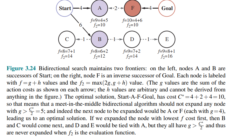
If an approach where the heuristic estimates the distance to the goal and estimates the distance to the start, it is called front-to-end search.

An alternative called front-to-front search attempt to estimate the distance to the other frontier. Clearly, if a frontier has millions of nodes, it would be inefficient to apply the heuristic function to every one of them and take the minimum.

Bidirectional search is sometimes more efficient than unidirectional search, sometimes not.

---

🧩 Summary of A star variants

Algorithm	Key idea	Key trade-off	Complete?	Optimal?	Optimal efficiency?
IDA*	Iterative DFS with increasing f-cost cutoff	Very low memory, but repeated full re-search	Yes (finite branching, positive costs)	Yes (with admissible heuristic)	No
RBFS	DFS guided by f, uses -limit + backed-up values	Linear memory, but frequent re-expansion of nodes	Yes (with admissible heuristic)	Yes (with admissible heuristic)	No
SMA*	A* with fixed memory; deletes worst -leaf when full	Best use of available memory, but possible thrashing	Yes (if solution fits memory depth)	Yes (if optimal solution fits memory)	Yes (within memory limits)
A*	Expands lowest , keeps full frontier	High memory usage, exponential growth	Yes (positive costs, finite branching)	Yes (with admissible heuristic)	Yes (with consistent heuristic)
Weighted A*	, inflates heuristic to speed up search	Faster search, loses optimality guarantee	Yes (typically)	No (bounded suboptimal)	No
Greedy best-first	Expands lowest only	Very fast, ignores path cost	No (in general)	No	No
Beam search	Keeps only top-k nodes per level	Strong memory control, but may discard solution	No	No	No
Bidirectional heuristic search	Search from start and goal simultaneously	Reduces depth exponentially, complex coordination	Yes (with proper conditions)	Yes (with admissible heuristics)	No (no guarantee)

---

Heuristic Functions

The accuracy of a heuristic affects the search performance.

Consider the 8-puzzle with reachable states, usually a search could easily keep them all in memory. But for the 15-puzzle there are states with over 10 trillion possible states.

There is a long history of such heuristics for the 15-puzzle; here are two commonly used candidates:

• : the number of misplaced tiles.
• : the sum of the distances of the tiles from their goal positions. Since tiles cannot move along diagonals, the distance is the sum of the horizontal and vertical distances, sometimes called the city-block distance or Manhattan distance.

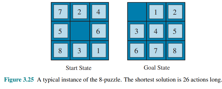
• is admissible because any tile that is out of place will require at least one move to get it to the right place.
• is the sum of the distances of the tiles from their goal positions. It is admissible because all any move can do is move one tile one step closer to the goal. Tiles 1 to 8 in the start state of figure 3.25 give a Manhattan distance of: that is less than the true solution cost of 26.

🧩 The effect of heuristic accuracy on performance

One way to characterize the quality of a heuristic is the effective branching factor .

If the total number of nodes generated by for a particular problem is and the solution depth is , then is the branching factor that a uniform tree of depth would have to have in order to contain nodes. Thus:

For example, if finds a solution at depth 5 using 52 nodes, then the effective branching factor is 1.92.

A better way to characterize the effect of pruning with a given heuristic is that it reduces the effective depth by a constant compared to the true depth.

This means that the total search cost is compared to for an uninformed search.

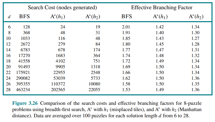
If one heuristic’s value is greater than or equal to another for all states (and strictly greater for some), we say that it dominates the other. In our case, dominates .

🧩 Generating Heuristics from relaxed problems

A problem with fewer restrictions on the actions is called a relaxed problem.

The state-space graph of the relaxed problem is a supergraph of the original state space because the removal of restrictions creates added edges. Therefore, any optimal solution to the original problem is by definition also a solution to the relaxed problem. However, the relaxed problem may have better (shorter) solutions if the added edges provide shortcuts. Hence, the cost of an optimal solution to a relaxed problem is an admissible heuristic for the original problem.

Relaxed problem = easier problem ⇒ lower optimal cost ⇒ admissible heuristic.

If a problem definition is written in a formal language, it is possible to construct relaxed problems automatically. For example, if the 8-puzzle actions are described as:

A tile can move from square X to square Y if
X is adjacent to Y and Y is blank

We can generate three relaxed problems by removing one or both of the conditions:

1. A tile can move from square X to square Y if X is adjacent to Y. (leads to , Manhattan distance)
2. A tile can move from square X to square Y if Y is blank.
3. A tile can move from square X to square Y. (leads to , misplaced tiles)

Notice that it is crucial that the relaxed problems generated by this technique can be solved essentially without search, because the relaxed rules allow the problem to be decomposed into independent subproblems.

If a collection of admissible heuristics is available for a problem, we can choose the best as:

This composite heuristic picks whichever function is most accurate on the node in question. dominates all its component heuristics. The only drawback is the longer computation time. If that is an issue, it is possible to randomly select one of the heuristics or use a Machine Learning algorithm to predict which will be the best.

🧩 Generating Heuristics from Subproblems: Pattern databases

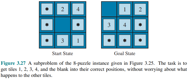
The idea behind pattern databases is to store exact solution costs for every possible subproblem instance. In this example, every possible configuration of four tiles and the blank would be stored. In total there will be patterns in the database. Then we compute an admissible heuristic for each state encountered during a search simply by looking up the corresponding subproblem configuration in the database.

The database itself is constructed by searching back from the goal and recording the cost of each new pattern encountered. The expense of this search is amortized over subsequent problem instances.

Each database yields an admissible heuristic, and these can be combined by taking the maximum value.

If we want to sum the costs, we need to ensure they don’t overlap in terms of moves. This leads to the idea of disjoint pattern databases. By recording only the moves involving the specific tiles of the subproblem, the total cost becomes a lower bound on the cost of solving the entire problem.

With such databases, it is possible to solve a 15-puzzle in a few milliseconds.

🧩 Generating Heuristics with landmarks

Route-finding services use precomputation of optimal path costs. This is time-consuming but needs only be done once and is amortized over billions of user requests.

We could generate a perfect heuristic by precomputing the cost of the optimal path between every pair of vertices, but that would require space.

A better approach is to choose a few landmark points (also called pivots or anchors) from the vertices. For each landmark and for each vertex in the graph, we compute and store , the exact cost of the optimal path from to .

Given the stored tables, we can create an efficient (though potentially inadmissible) heuristic:

If the optimal path goes through a landmark, this heuristic will be exact; otherwise, it may overestimate the cost (inadmissible).

Some route-finding algorithms save even more time by adding shortcuts, which are artificial edges in the graph that define an optimal multi-action path.

is efficient but not admissibile, an heuristic that is both efficient and admissible would be:

That is called differential heuristic (because of the subtraction).

Consider for example a landmark that is somewhere out beyond the goal. If the goal happens to be on the optimal path from to the landmark, this is as saying:

“Consider the entire path from to , then subtract off the last part of that path, from goal to , giving us the exact cost of the path from to goal”

The goal will still be a bit off the optimal path to the landmark, the heuristic will be inexact but still admissible. Landmarks that are not out beyond the goal will not be useful.

There are several ways to pick landmark points:

Random: Selecting random point is fast but it is better to spread the landmarksout so they are not too close to each other. A greedy approach is to pick a first landmark at random, then find the point that is furthest from that, and add it to the set of landmarks, and continue, at each iteration adding the point that maximizes the distance to the nearest landmark.

Past search requests: if you have logs of past search requests, then you can pick landmarks that are frequently requested in searches.

For the differential heuristic it is good if the landmarks are spread around the perimeter of the graph. Thus a good technique is to find the centroid of the graph, arrange pie-shaped wedges around the centroid, and in each wedge select the vertex that is the farthest from the center.

🧩 Learning to search better

An agent could learn how to search better, and this method rests on an important concept called metalevel state space. Each state in a metalevel state space captures the internal state of a program that is searching in an ordinary state space such as the map of Romania.

For example, the internal state of the algorithm consists of the current search Object-level state space tree. Each action in the metalevel state space is a computation step that alters the internal state.

For example, consider figure we saw in A* Search:

This figure shows a sequence of larger nad larger search trees, these can be seen as depcting a path in the metalevel state space where each state on the path is an object-level search tree.

The path in the figure has only 5 steps, including one that is not especially helpful. But consider an harder problem i.e with much more misssteps; a metalevel learning algorithm can learn from these experiences to avoid exploring unpromising subtrees. The goal is to minimize the total cost of problem solving, trading off computational expense and path cost.

🧩 Learning Heuristics from experience

We have seen that one way to invent a heuristic is to devise a relaxed problem for which an optimal solution can be found easily. An alternative is to learn from experience.

For example consider as “experience” solving lots of 8-puzzles. Each optimal solution to an 8-puzzle problem provides an example (goal, path) pair. From these examples, a learning algorithm can be used to construct a function that can (with luck) approximate the true path cost for other states that arise during search.

Most of these approaches learn an imperfect approximation to the heuristic function, and thus risk inadmissibility. Usually machine learning and in particular reinforcement learning methods are used.

Some machine learning techniques work better when supplied with features of a state that are relevant to predicting the state’s heuristic value, rather than with just the raw state description. For example, the feature “number of misplaced tiles” might be helpful in predicting the actual distance of an 8-puzzle state from the goal.

We could take 100 randomly generated 8-puzzle configurations and gather statistics on their actual solution costs.

The most simple approach is using a linear combination:

where constants and are adjusted to give the best fit to the actual data across the randomly generated configurations.

Notice that this heuristic satisfies the condition for goal states, but it is not necessarily admissible or consistent.