AI - Lecture - Solving Problems by Searching - Adversarial Search and Games
- Source: Book Artificial Intelligence A Modern Approach 4 edition global edition - Russel - Chapter 6
In a competitive environments two or more agents have conflicting goals, giving rise to adversarial search problems. We can consider games like chess, Go, and poker.
For AI researchers, the simplified nature of these games is a plus: the state of a game is easy to represent, and agents are usually restricted to a small number of actions whose effects are defined by precise rules. Physical games, such as croquet and ice hockey, have more complicated descriptions, a larger range of possible actions, and rather imprecise rules defining the legality of actions.
Game Theory
There are at least three stances we can take towards multi-agent environments.
When there are a very large number of agents, we need to consider them in the aggregate as an economy, allowing us to do things like predict that increasing demand will cause prices to rise, without having to predict the action of any individual agent.
See also
- Patchwork AGI hypothesis for a discussion about the implications of an economy of AI agents
Second we need to consider adversarial agents as just a part of the environment -part that makes the environment nondeterministic. But if we model the adversaries in the same way that, say, rain sometimes falls and sometimes doesn’t, we miss the idea that our adversaries are actively trying to defeat us, whereas the rain supposedly has no such intention
The third stance is to explicitly model the adversarial agents with the techniques of adversarial game-tree search. We start by considering the minimax search that is a generalisation of AND-OR search tree. Pruning makes the search more efficient by ignoring portions of the search tree that makes no difference to the optimal move.
For each state where we choose to stop searching, we ask who is winning. To answer this question we have a choice: we can apply a heuristic evaluation function to estimate who is winning based on features of the state, or we can average the outcomes of many fast simulations of the game from that state all the way to the end.
Two-player zero-sum games
The games most commonly studied within AI are what game theorists call deterministic, two-player, turn-taking, perfect information, zero-sum games.
Perfect Information is a synonym for fully observable. Zero-sum means that what is good for one player is just as bad for the other: there is no “win-win” outcome.
For games we often use the term move as a synonym for “action” and a position as a synonym for “state”.
We consider two players MAX and MIN. MAX moves first, and then the players take turns moving until the game is over. At the end of the game, points are awarded to the winning player and penalties are given to the loser.
Formally a game has the following elements:
is the initial state which specifies how the game is set up at the start - TO-MOVE(s): the player whose turn it is to move into state s.
- ACTIONS(s) is the set of legal moves in state s
- RESULT(s,a) is the transition model, which defines the state resulting from taking action a in state s
- IS-TERMINAL(s): a terminal test, which is true when the game is over and false otherwise. States where the game has ended are called terminal states.
- UTILITY(s,p): a utility function (also called an objective function or payoff function), which defines the final numeric value to player p when the game ends in the terminal state s. In chess, the outcome is win, loss or draw, with values 1, 0 or
. Some games have a wider range of possible outcomes for example the payoff in backgammon range from 0 to 192.
Tic-tac-toe instantiation
initial state → empty board - player to move → X/O to move - legal actions → empty cells - successor state → board after placing a mark - terminal-state test → Win/loss/draw - payoff at terminal states → +1, 0, -1
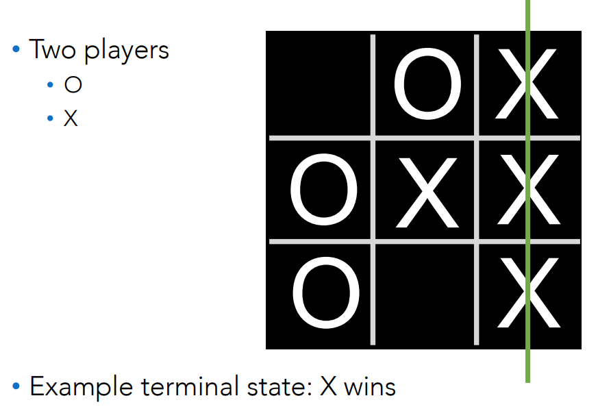
The initial state, ACTIONS function and RESULT function define the state space graph a graph where:
- the vertices are states
- the edges are moves
- a state might be reached by multiple paths.
A search tree over part of that graph to determine what move to make. We define the complete game tree as a search tree that follows every sequence of moves all the way to a terminal state. The game tree may be infinite if the state space itself is unbounded or if the rules of the game allow for infinitely repeating positions.
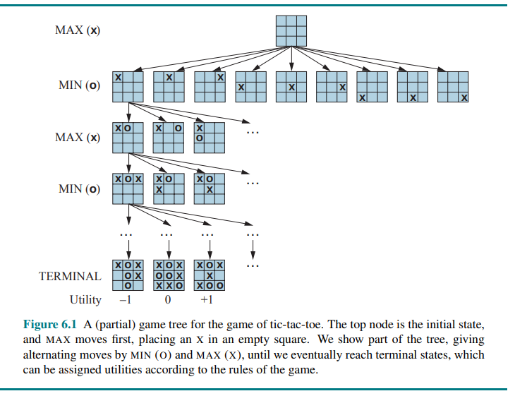
For tic-tac-toe the game tree is relatively small, fewer than
Types of games
Games can be classified along two dimensions:
- information available to the players
- presence of randomness

Optimal Decisions in Games
- MAX wants to find a sequence of actions leading to a win.
- MIN wants to prevent it.
This means that MAX’s strategy must be a conditional plan i.e. a contingent strategy specifying response to each of MIN’s possible moves.
In previous lesson we talked about conditional plan in a non-deterministic environment. A multi-agent environment is non-deterministic because of the presence of multiple agents
Contingent Strategy
A contingent strategy (or contingency strategy) is a flexible approach where an organization adapts its actions based on specific internal or external situations, as there is no single “best” way to manage or lead. This concept, rooted in contingency theory, asserts that optimal decisions depend entirely on the current context, requiring leaders to be agile rather than rigid in their methods.
In games with a binary outcome (win or lose), we could use AND-OR search to generate the conditional plan. In fact, for such games, the definition of a winning strategy for the game is identical to the definition of a solution for a nondeterministic planning problem: in both cases the desirable outcome must be guaranteed no matter what the “other side” does.
For games with multiple outcome scores, we need a slightly more general algorithm called minmax search.
Minimax key concepts
- minimax applies to two-player, zero-sum, deterministic game
- both players are assumed to play optimally
- the game tree is evaluated recursively until terminal states are reached
- terminal stated are assigned a utility values (for example -1, 0, 1 in tic-tac-toe)
- MAX chooses the action with the highest value, while MIN chooses the action with the lowest value
- Internal nodes are evaluated by propagating these utilities upward
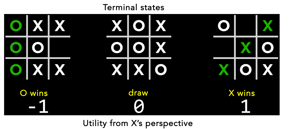
Consider a trivial game like this:
The possible moves are
The value of a state depends on the future choices of both players:
- At a MAX node, we select the child with the highest value
- At a MIN node, we select the child with the lowest value
Hence, values are computed recursively by alternating MAX and MIN levels
In some games, the word “move” means that both players have taken an action; therefore the word ply is used to unambiguously mean one move by one player, bringing us one level deeper in the game tree.
Given a game tree, the optimal strategy can be determined by working out the minimax value of each state in the tree, which we write as MINIMAX(s). The minimax value is the utility (for MAX) of being in that state, assuming that both players play optimally from there to the end of the game.
The minimax value of a terminal state is just its utility. In a nonterminal state, MAX prefers to move to a state of maximum value when it is MAX’s turn to move, and MIN prefers a state of minimum value (that is, minimum value for MAX and thus maximum value for MIN). So we have:
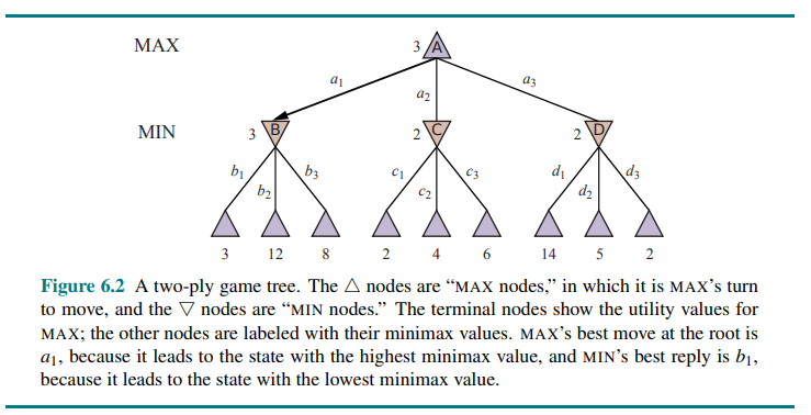
Let’s apply these definitions to the game tree in Figure 6.2.
The terminal nodes on the bottom level get their utility values from the game’s UTILITY function. The first MIN node, labeled B has three successor states with values 3, 12, and 8, so its minimax value is 3.
Similarly, the other two MIN nodes have minimax value 2.
The root node is a MAX node; its successor states have values 3, 2 and 2, so it has a minimax value of 3.
We can also identify the minimax decision at the root: action
This definition of optimal play for MAX assumes that MIN also plays optimally.
What if MIN does not play optimally?
Then MAX will do at least as well as against an optimal player, possibly better. Does not mean that it is always best to play the minimax optimal move when facing a suboptimal opponent.
For example, in a situation where optimal play by both sides will lead to a draw, but there is one risky move for MAX that leads to a state in which there are 10 possible response moves by MIN that all seem reasonable, but 9 of them are a loss for MIN and one is a loss for MAX.
If MAX believes that MIN does not have sufficient computational power to discover the optimal move, MAX might want to try the risky move on the grounds that a 9/10 chance of a win is better than a certain draw.
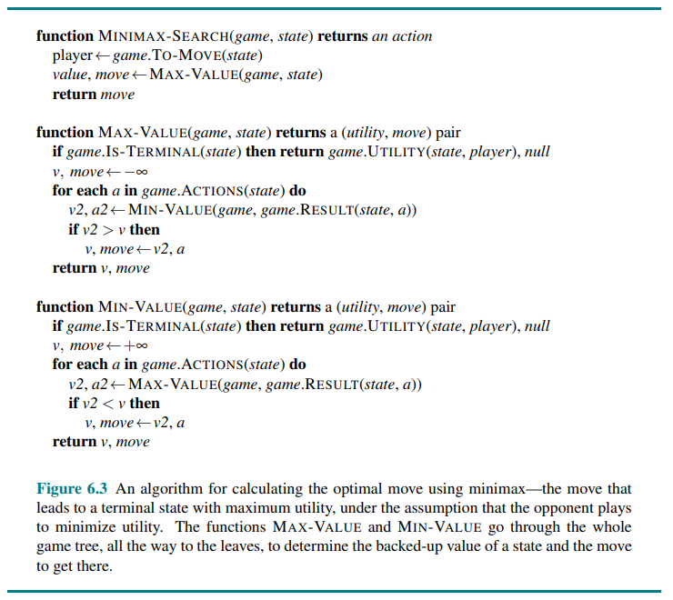
Minimax search algorithm
Minimax complexity
The minimax algorithm performs a complete depth-first exploration of the game tree.
- Time complexity:
- Space complexity:
- where
=branching factor, =maximum depth of the search tree
The exponential complexity makes MINIMAX impractical for complex games; for example, chess has a branching factor of about 35 and the average game has a depth of about 80 ply, and it is not feasible to search
By approximating the minimax analysis in various ways, we can derive more practical algorithms.
We need more efficient methods, starting with alpha-beta pruning.
Optimal decisions in multiplayer games
Many popular games allow more than two players.
To extend this concept to multiplayer games, first replace the single value for each node with a vector of values. For example, in a three-player game, with players A, B and C, a vector
The simplest way to implement this is to have the UTILITY function return a vector of utilities.
Now we have to consider nonterminal states. Consider the node marked 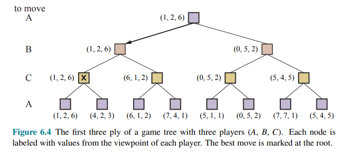
In that state, player
Anyone who plays multiplayer games, such as Diplomacy or Settlers of Catan, quickly becomes aware that much more is going on than in two-player games.
Multiplayer games usually involve alliances, whether formal or informal, among the players. Alliances are made and broken as the game proceeds. How are we to understand such behavior? Are alliances a natural consequence of optimal strategies for each player in a multiplayer game? It turns out that they can be.
For example if A and B are in weak positions and C is in stronger position, then it is often optimal for both A and B to attack C rather than each other, lest C destroy each of them individually. Of course, as soon as C weakens under the joint onslaught, the alliance loses its value, and either A or B could violate the agreement.
If the game is not zero-sum, then collaboration can also occur with just two players. Then the optimal strategy is for both players to do everything possible to reach this state i.e. cooperate to achieve a mutually desirable goal.
Alpha-Beta Pruning
Since the number of game states is exponential in the depth of the tree, no algorithm can completely eliminate the exponent, but we can sometimes cut it in half, computing the correct minimax decision without examining every state by pruning. (See A* pruning).
In particular what is called the alpha-beta pruning.
Recall that:
- Plain minimax evaluates the game tree bottom-up from the leaves
- every internal node is assigned a value by applying min or max to its children
- To determine the root value, minimax explores all branches of the tree
Intuition: the idea behind alpha-beta pruning is that once a branch is known to be unable to improve the current minimax decision, it does not need to be explored further. Alpha-beta pruning improves minimax by eliminating branches that are provably irrelevant.
Consider again the two-ply game tree:
Let’s go through the calculation of the optimal decision once more, this time paying careful attention to what we know at each point in the process.
The steps are explained in the following figure:
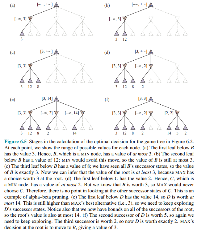
So the outcome is that we can identify the minimax decision without ever evaluating two of the leaf nodes. Another way to look at this is a simplification of the formula for MINIMAX.
Let the two unevaluated successors of node
In other words, the value of the root and hence the minimax decision are independent of the values of the leaves
Alpha–beta pruning can be applied to trees of any depth, and it is often possible to prune entire subtrees rather than just leaves.
The general principle is this: consider a node
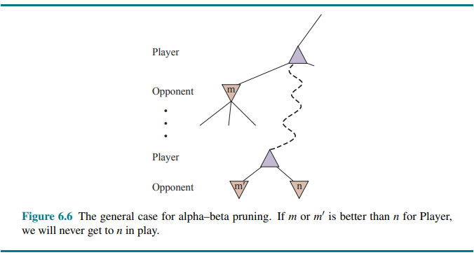
Minimax search is depth-first, so at any time we just have to consider the nodes along a single path in the tree.
A branch is pruned when it cannot change the value returned by the current node. This reduces the search cost while preserving correctness. Therefore, alpha-beta pruning returns the same minimax value as exhaustive search.
Alpha-beta pruning gets its name from the two extra parameters in MAX-VALUE(state,
: the value of the best (highest-value) choice we have found so far at any choice point along the path for MAX. Think: = “at least”. : the value of the best (lowest-value) choice we have found so far at any choice point along the path for MIN. Think: = “at most”.
Alpha-beta pruning example
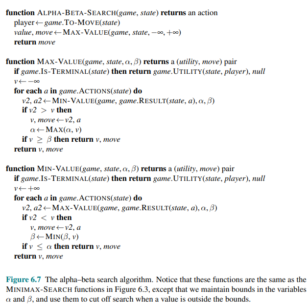
- Consider this tree:
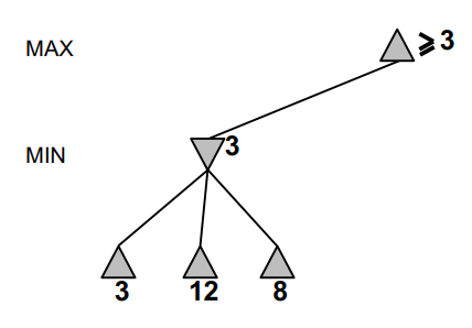
- The first explored subtree returns value 3. At the root, MAX now knows that it can guarantee a value of atleast 3. Therefore, the current lower bound is
. 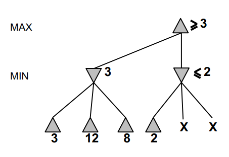
- In the next MIN subtree, the first child gives value 2, so
- Since:
this MIN subtree cannot produce a value better than the alternative already available to the current MAX ancestor. The remaining children can therefore be pruned. 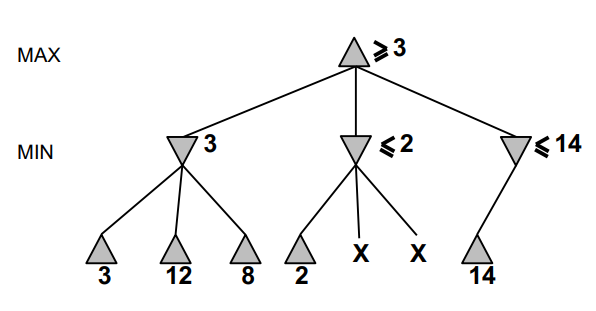
- Now we have a lower bound of 3 and an upper bound
. Since we do not have that we cannot prune this subtree. 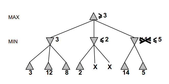
- After exploring the children of the MIN node, we have that the upper bound becomes
- This is a tighter bound than before, but we still do not have
, so no pruning is possible yet. 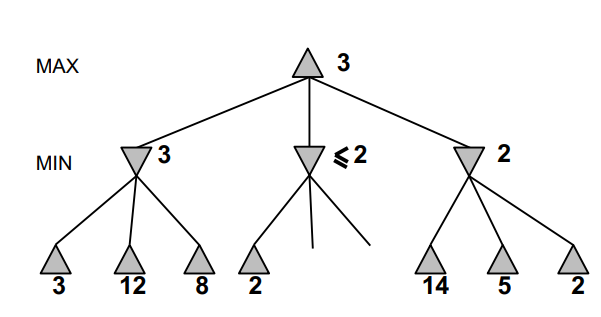
- Final result: the left subtree establishes a best value of 3 for the root.
- In the middle MIN subtree, the first explored child has value 2, so
- Therefore the remaining children of that subtree cannot affect the root decision and can be pruned
Key point: alpha-beta pruning returns the same minimax value with fewer node evaluations.
Properties of the alpha-beta
- Alpha-beta is exact: it returns the same minimax value as full minimax
- Its effectiveness depends strongly on the order in which moves are explored
- With perfect move ordering, the best-case time complexity improves from
to . - This allows the search to reach roughly twice the depth in the same amount of time.
- Even with this improvement, exhaustive search remains infeasible in games such as chess
Move ordering
The effectiveness of alpha–beta pruning is highly dependent on the order in which the states are examined.
Consider step (e) and (f) of:
We could not prune any successors of
If this could be done perfectly, alpha-beta would need to examine only
We cannot get the perfect move ordering, in that case the ordering function could be used to play a perfect game. But we can often get fairly close, it depends on the game. For example in chess a fairly simple ordering function gets you to within about a factor of 2 of the best-case
Adding dynamic move-ordering schemes, such as trying first the moves that were found to be best in the past, brings us quite close to the theoretical limit.
The past could be the previous move—often the same threats remain—or it could come from previous exploration of the current move through a process of iterative deepening.
The best moves are known as killer moves, and to try them first is called the killer move heuristic.
We noted that redundant paths to repeated states can cause an exponential increase in search cost, and that keeping a table of previously reached states can address this problem.
In game tree search, repeated states can occur because of transposition i.e. different permutations of the move sequence that end up in the same position, and the problem can be solved with transposition table that caches the heuristic value of states.
Even with alpha–beta pruning and clever move ordering, minimax won’t work for games like chess and Go, because there are still too many states to explore in the time available.
Historically Shannon in his very first paper on computer game playing, Programming a Computer for Playing Chess (Shannon, 1950), Claude Shannon recognized this problem and proposed two strategies:
- Type A strategy considers all possible moves to a certain depth in the search tree, and then uses a heuristic evaluation function to estimate the utility of states at that depth. It explores a wide but shallow portion of the tree.
- Type B strategy ignores moves that look bad, and follows promising lines “as far as possible.” It explores a deep but narrow portion of the tree.
Historically, most chess programs have been Type A whereas Go programs are more often Type B because the branching factor is much higher in Go.
Mnemonic cheat sheet
- Standard minimax explores every state in the game and has an exponential complexity
- Alpha-Beta pruning tries to prune some of these states by pruning tree branches that mathematically we know they won’t lead to a better result (so that children of these nodes are never considered)
- Alpha-Beta name come from his two parameters:
and - A rational MAX player will consider only moves that gives atleast
- A rational MIN player will consider only moves that gives atmost
- Everytime we go one layer down in the tree, these values are updated. If
then we have to prune that subtree - The efficiency of alpha-beta pruning depends on the move ordering, game-specific heuristics are used
- Alpha beta with a good heuristic improves complexity from
to - To make the algorithm computationally maneagable (however not anymore exact) you cut the maximum depth to a fixed value
Depth limited minimax
Practical adversarial search rarely reaches the leaves of the full game tree. Instead, search is truncated at a predefined depth
- Terminal states return their exact utility
- Non-terminal states at depth
are evaluated by an evaluation function
Consequence: the algorithm is no longer exact, but it becomes computationally manageable.
An evaluation function assigns a heuristic value to a non-terminal state.
It is used when depth-limited search stops before reaching a terminal state. Its purpose is to approximate the true utility of the position
The better the evaluation function, the better the decisions made by the search algorithm. For example in chess we may interpret values as:
- +1 white wins
- 0 draw
- -1 black wins
A score of 0.8 indicates that White is strongly favored but not guaranteed to win.
In games such as chess, a state is often evaluated through a set of descriptive features. A common form is a weighted sum of those features:
The features capture relevant properties of the position, such as: material balance, mobility, king safety, pawn structure.
Example
Modern game-playing systems often learn
🧩 Heuristic Alpha-Beta Tree Search
To make use of our limited computation time, we can cut off the search early and apply a heuristic evaluation function to states, effectively treating nonterminal nodes as if they were terminal. In other words we replace the UTILITY function with EVAL which estimates a state’s utility. We also replace the terminal test by a cutoff test, which must return true for terminal states, but is otherwise free to decide when to cut off the search, based on the search depth and any property of the state that it chooses to consider.
That gives us the formula H-MINIMAX(s,d) for the heuristic minimax value of state
Evaluation Functions
An evaluation function assigns a heuristic value to a non-terminal state. The better the evaluation function, the better the decisions made by the search algorithm.
For example, in chess we may interpret values as:
- +1 white wins
- 0 draw
- -1 black wins
A score of 0.8 indicates that white is strongly favoured, but not guaranteed to win.
In a game like chess usually evaluation functions works by calculating various features of the state like the number of white pawns, black pawns, white queens, black queens and so on. For example, one category might contain all two-pawn versus one-pawn endgames.
The evaluation function does not know which states are which, but it can return a single value that estimates the proportion of states with each outcome.
For example suppose our experience suggests that
A reasonable evaluation for states in the category is the expected value:
In practice, this kind of analysis requires too many categories and hence too much experience to estimate all the probabilities. Instead, most evaluation functions compute separate numerical contributions from each feature and then combine them to find the total value.
For centuries chess players have developed ways of judging the value of a position using just this idea. For example, introductory chess books give an approximate material value for each piece:
- each pawn is worth 1,
- a knight or bishop is worth 3,
- a rook 5,
- and the queen 9.
- Other features such as “good pawn structure” and “king safety” might be worth half a pawn, say.
These features values are then simply added up to obtain the evaluation of the position. Mathematically, this kind of evaluation function is called a weighted linear function because it can be expressed as:
- where each
is a feature of the position (such as “number of white bishops”) and each is a weight (saying how important that feature is).
The weights should be normalized so that the sum is always within the range of a loss (0) to a win (+1).
We said that the evaluation function should be strongly correlated with the actual chances of winning, but it need not be linearly correlated: if state
Adding up the values of features seems like a reasonable thing to do, but in fact it involves a strong assumption: that the contribution of each feature is independent of the values of the other features. For this reason, current programs for chess and other games also use nonlinear combinations of features. For example, a pair of bishops might be worth more than twice the value of a single bishop, and a bishop is worth more in the endgame than earlier—when the move number feature is high or the number of remaining pieces feature is low.
Where do the features and weights come from? They’re not part of the rules of chess, but they are part of the culture of human chess-playing experience. In games where this kind of experience is not available, the weights of the evaluation function can be estimated by the machine learning. Applying these techniques to chess has confirmed that a bishop is indeed worth about three pawns.
Cutting off search
The next step is to modify the ALPHA-BETA-SEARCH so that it will call the heuristic EVAL function when it is appropriate to cut off the search.
We replace the two lines in Figure 6.7:
that mention IS-TERMINAL with the following line: if game.IS-CUTOFF(state, depth) then return game.EVAL(state, player), null.
We also must arrange for some bookkeeping so that the current depth is incremented on each recursive call. The most straightforward approach is to set a fixed depth limit such that IS-CUTOFF(state, depth) returns true for all depth greater than some fixed depth
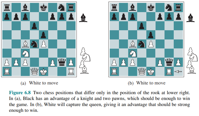
These simple approaches can lead to errors due to the approximate nature of the evaluation function. Consider again the simple evaluation function for chess based on material advantage.
Suppose the program searches to the depth limit, reaching the position in Figure 6.8(b), where Black is ahead by a knight and two pawns.
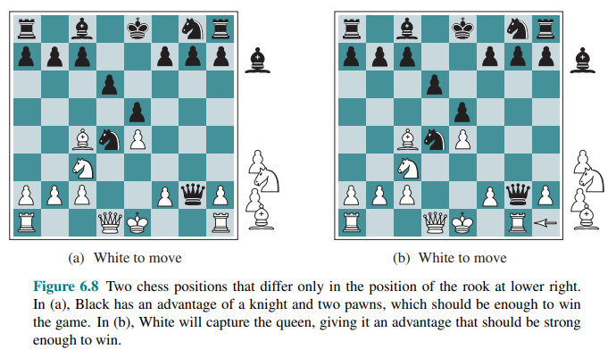
It would report this as the heuristic value of the state, thereby declaring that the state is a probable win by Black. But White’s next move captures Black’s queen with no compensation. Hence, the position is actually favorable for White, but this can be seen only by looking ahead.
The evaluation function should be applied only to positions that are quiescent: that is positions in which there is no pending move (such as a capturing the queen) that would wildly swing the evaluation.
For nonquiescent positions the IS-CUTOFF returns false, and the search continues until quiescent positions are reached. This extra quiescence search is sometimes restricted to consider only certain types of moves, such as capture moves, that will quickly resolve the uncertainties in the position.
The horizon effect is more difficult to eliminate. It arises when the program is facing an opponent’s move that causes serious damage and is ultimately unavoidable, but can be temporarily avoided by the use of delaying tactics.
Consider the chess position in Figure 6.9:
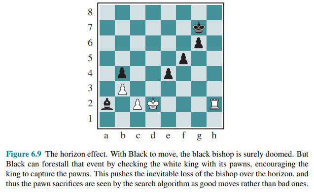
One strategy to mitigate the horizon effect is to allow singular extensions, moves that are “clearly better” than all other moves in a given position, even when the search would normally be cut off at that point. This makes the tree deeper, but because there are usually few singular extensions, the strategy does not add many total nodes to the tree, and has proven to be effective in practice.
Forward pruning
Alpha–beta pruning prunes branches of the tree that can have no effect on the final evaluation, but forward pruning prunes moves that appear to be poor moves, but might possibly be good moves. Thus, the strategy saves computation time at the risk of making an error. (Type B strategy) Clearly, most human chess players do this, considering only a few moves from each position (at least consciously).
One approach to forward pruning is beam search: on each ply, consider only a “beam” of the
Another approach is a probabilistic cut, the PROBCUT that is a forward-pruning version of alpha-beta search that uses statistics gained from prior experience to lessen the chance that the best move will be pruned. Alpha-beta search prunes any node that is provably outside the current
Another technique, late move reduction, works under the assumption that move ordering has been done well, and therefore moves that appear later in the list of possible moves are less likely to be good moves. But rather than pruning them away completely, we just reduce the depth to which we search these moves, thereby saving time. If the reduced search comes back with a value above the current
Performance:
Combining all the techniques described here results in a program that can play creditable chess (or other games).
However, we can generate and evaluate around a million nodes per second on the latest PC. The branching factor for chess is about 35, on average, and
With alpha-beta search and a large transposition table we get to about 14 ply, which results in an expert level of play.
To obtain the grandmaster status we would still need an extensively tuned evaluation function and a large database of endgame moves. Top chess programs like STOCKFISH have all of these, often reaching depth 30 or more in the search tree and far exceeding the ability of any human player.
Search vs lookup
Somehow it seems like overkill for a chess program to start a game by considering a tree of a billion game states, only to conclude that it will play pawn to e4 (the most popular first move).
Many gameplaying programs use table lookup rather than search for the opening and ending of games.
For the openings, the computer is mostly relying on the expertise of humans. The best advice of human experts on how to play each opening can be copied from books and entered into tables for the computer’s use. In addition, computers can gather statistics from a database of previously played games to see which opening sequences most often lead to a win. After about 10 or 15 moves we end up in a rarely seen position, and the program must switch from table lookup to search.
Near the end of the game there are again fewer possible positions, and thus it is easier to do lookup. But here it is the computer that has the expertise: computer analysis of endgames goes far beyond human abilities. A king-and-rook-versus-king endgame is easy to win, but other endings like king, bishop and knight versus king (KBNK) are difficult to master and have no succinct strategy description.
A computer, on the other hand, can completely solve the endgame by producing a policy which is a mapping from every possible state to the best move in that state. Then the computer can play perfectly by looking up the right move in this table. The table is constructed by retrograde minimax search: start by considering all ways to place the KBNK pieces on the board. Some of the positions are wins for white; mark them as such. Then reverse the rules of chess to do reverse moves rather than moves. Any move by White that, no matter what move Black responds with, ends up in a position marked as a win, must also be a win. Continue this search until all possible positions are resolved as win, loss, or draw, and you have an infallible lookup table for all endgames with those pieces. This has been done not only for KBNK endings, but for all endings with seven or fewer pieces. The tables contain 400 trillion positions. An eight-piece table would require 40 quadrillion positions.
Monte Carlo Tree Search
The game of Go illustrates two major weakness of heuristic alpha-beta tree search:
- First, Go has a branching factor that starts at 361, which means alpha-beta search would be limited to only 4 or 5 ply.
- Second, it is difficult to define a good evaluation function for Go because material value is not a strong indicator and most positions are in flux until the endgame.
In response to these two challenges, modern Go programs have abandoned alpha–beta search and instead use a strategy called Monte Carlo tree search (MCTS).
The basic MCTS strategy does not use a heuristic evaluation function, instead the value of a state is estimated as the average utility over a number of simulations of complete games starting from the state. A simulation (also called a playout or rollout) chooses moves first for one player, then for the other, repeating until a terminal position is reached.
MCTS estimates move quality through sampling, rather than exhaustive search.
At that point the rules of the game (not fallible heuristics) determine who has won or lost, and by what score. For a game with only win or loss outcomes, average utility is the same as win percentage.
To get useful information from the playout we need a playout policy that biases the moves towards good ones. For Go and other games, playout policies have been successfully learned from self-play by using neural networks. Sometimes game-specific heuristics are used, such as “consider capture moves” in chess or “take the corner square” in Othello.
Given a playout policy, we next need to decide two things: from what positions do we start the playouts, and how many playouts do we allocate to each position?
The simplest answer, called pure Monte Carlo search, is to do
For some stochastic games this converges to optimal play as
The core problem becomes how to balance exploration of uncertain moves and exploitation of moves that currently appear strong.
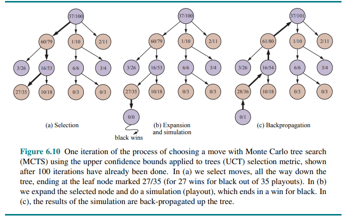
Monte Carlo tree search does that by maintaining a search tree and growing it on each iteration of the following four steps, as shown in Figure 6.10:
- Selection: choose successive child nodes from the root according to the selection policy
- Expansion: add a new child to the selected leaf
- Simulation: perform a playout from the new node
- Back-propagation: use the simulation result to update all nodes on the path to the root
Each node in a MCTS stores statistics from earlier playouts, typically win/visits.
During the selection step, MCTS starts from the root and repeatedly selects a child according to the selection policy. The traversal continues until a leaf or expandable node is reached.
Figure 6.10(a) shows a search tree with the root representing a state where white has just moved, and white has won 37 out of the 100 playouts done so far. The thick arrow shows the selection of a move by black that leads to a node where black has won 60/79 playouts. This is the best win percentage among the three moves; so selecting it is an example of exploitation. But it would also have been reasonable to select the 2/11 node for the sake of exploration—with only 11 playouts, the node still has high uncertainty in its valuation, and might end up being best if we gain more information about it.
Expansion: we grow the search tree by generating a new child of the selected node; Figure 6.10(b) shows the new node marked with 0/0.
Simulation: we perform a playout from the newly generated child node, choosing moves for both players according to the playout policy. These moves are not recorded in the search tree. In the figure, the simulation results in a win for black.
Back-propagation: we now use the result of the simulation to update all the search tree nodes going up to the root. Since black won the playout, black nodes are incremented in both the number of wins and the number of playouts, so 27/35 becomes 28/36 and 60/79 becomes 61/80. Since white lost, the white nodes are incremented in the number of playouts only, so 16/53 becomes 16/54 and the root 37/100 becomes 37/101.
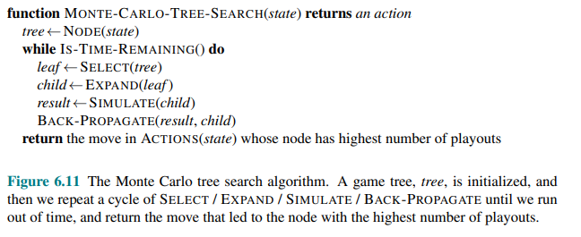
We repeat these four steps either for a set number of iterations, or until the allotted time has expired, and then return the move with the highest number of playouts.
One very effective selection policy is called “upper confidence bounds applied to trees” or UCT. The policy ranks each possible move based on an upper confidence bound formula called UCB1.
For a node
- where
is the total utility of all playouts that went through node , is the number of playouts through node , is the parent node of in the tree. is the exploitation term i.e. the average utility of . - The term with the square root is the exploration term: it has the count
in the denominator, which means the term will be high for nodes that have only been explored a few times. In the numerator it has the log of the number of times we have explored the parent of . - The constant
controls the balance between exploration and exploitation. In theory it should be but in practice game programmers try multiple values and choose the best performing one.
This means that if we are selecting
The time to compute a playout is linear, not exponential, in the depth of the game tree, because only one move is taken at each choice point.
For example: consider a game with a branching factor of 32, where the average game lasts 100 ply. If we have enough computing power to consider a billion game states before we have to make a move, then minimax can search 6 ply deep, alpha–beta with perfect move ordering can search 12 ply, and Monte Carlo search can do 10 million playouts. It is also possible to combine aspects of alpha–beta and Monte Carlo search. For example, in games that can last many moves, we may want to use early playout termination, in which we stop a playout that is taking too many moves, and either evaluate it with a heuristic evaluation function or just declare it a draw.
Monte Carlo search has a disadvantage when it is likely that a single move can change the course of the game, because the stochastic nature of Monte Carlo search means it might fail to consider that move. In other words, Type B pruning in Monte Carlo search means that a vital line of play might not be explored at all.
The general idea of simulating moves into the future, observing the outcome, and using the outcome to determine which moves are good ones is one kind of reinforcement learning.
When Monte Carlo Search is Useful
- In games with large branching factor like Go
- When strong evaluation functions are difficult to design
- When a more robust solution than alpha-beta is required. Monte Carlo Search estimates are based on many playouts rather than a single heuristic judgment
- MCST can be combined with heuristic functions to truncate some playouts.
- Monte Carlo can be applied to new games using only the game rules
- Strong policies can be learned through self-play (in fact is a kind of reinforcement learning)
Stochastic Games
Stochastic games bring us a little closer to the unpredictability of real life by including a random element, such as the throwing of dice. Backgammon is a typical stochastic game that combines luck and skill.
A game is stochastic when transitions between states are partly determined by chance. In addition to player decisions, the game includes random events that influence the outcome.
Typical sources of randomness include:
- chance variables, such as dice or card draws
- probabilistic action outcomes
This changes the search problem: instead of computing only max and min over successors, we must also compute expectations over random outcomes.
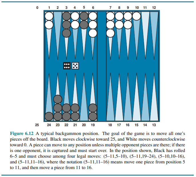 At this point Black knows what moves can be made, but does not know what White is going to roll and thus does not know what White’s legal moves will be. That means Black cannot construct a standard game tree of the sort we saw in chess and tic-tac-toe.
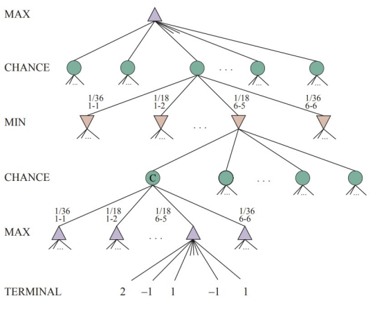
A game tree in backgammon must include chance nodes in addition to MAX and MIN nodes. They are shown in the following figure:
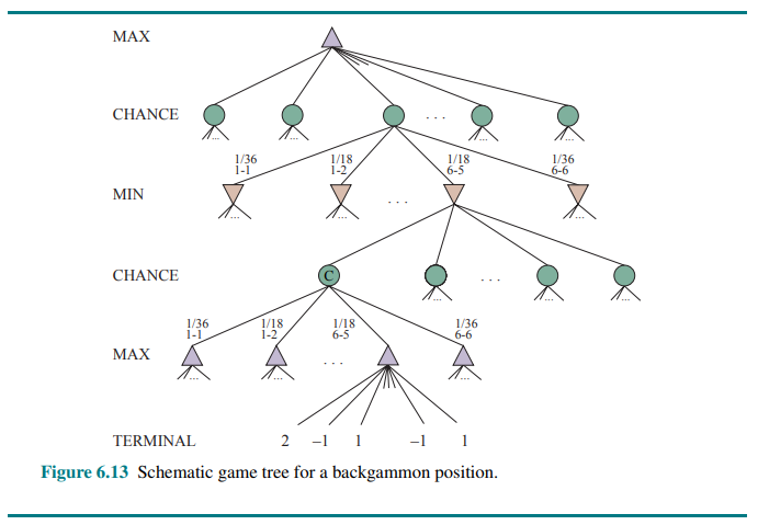 Chance nodes represents random events. After a player selects an action, a chance node determines the next state. Each branch from the chance node corresponds to a possible outcome and carries an associated probability.
Hence, a state-action pair defines a probability distribution over successor states. This can be interpreted as introducing a chance agent that acts after the players, but does not optimize any objective.
The branches leading from each chance node denote the possible dice rolls; each branch is labeled with the roll and its probability. There are 36 ways to roll two dice, each equally likely; but because a 6–5 is the same as a 5–6, there are only 21 distinct rolls. The six doubles (1–1 through 6–6) each have a probability of 1/36, so we say P(1–1) = 1/36. The other 15 distinct rolls each have a 1/18 probability.
The next step is to understand how to make correct decisions.
Obviously, we still want to pick the move that leads to the best position. However, positions do not have definite minimax values. Instead, we can only calculate the expected value of a position: the average over all possible outcomes of the chance nodes.
This leads us to the expectiminimax value for games with chance nodes, a generalization of the minimax value for non-deterministic games.
Terminal nodes and MAX and MIN nodes work exactly the same way as before (with the caveat that the legal moves for MAX and MIN will depend on the outcome of the dice roll in the previous chance node).
For chance nodes we compute the expected value, which is the sum of the value over all outcomes, weighted by the probability of each chance action:
where
In stochastic games, the value of a state depends on both adversarial choices and random outcomes. Minimax is therefore extended by replacing chance nodes with expected values.
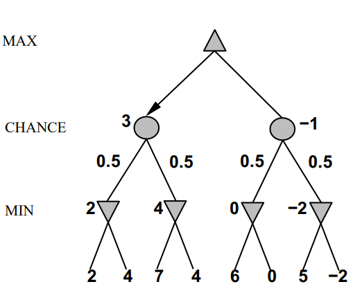
Expectiminimax simplified example - coin-flipping
- MIN nodes take the minimum of their children
- CHANCE nodes compute the expected value of their children
- Since the coin is fair, each outcome has probability 0.5
- The root is a MAX node, so it selects the branch with value 3
Evaluation functions for game of chance
As with minimax, the obvious approximation to make with expectiminimax is to cut the search off at some point and apply an evaluation function to each leaf.
The difference with alpha-beta is that chance nodes must combine the values of successor states through expectation. Therefore, in stochastic games, the actual numeric values matter, not only their ordering.
Important consequence:
- In minimax, preserving the ranking of states is enough
- In expectiminimax, the evaluation function should be a positive linear transformation of the true expected utility
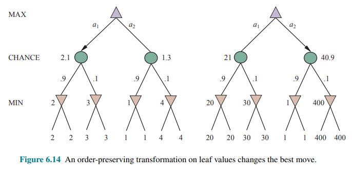
- At chance nodes, values are averaged
- Therefore, changing the numerical scale of evaluation values can change the preferred decision, even when the rank order of leaves stays the same.
With an evaluation function that assigns the values
It turns out that to avoid this problem, the evaluation function must return values that are a positive linear transformation of the probability of winning (or of the expected utility, for games that have outcomes other than win/lose). This relation to probability is an important and general property of situations in which uncertainty is involved.
Complexity:
If the program knew in advance all the dice rolls that would occur for the rest of the game, solving a game with dice would be just like solving a game without dice, which minimax does in
Complexity - example: In backgammon
Pruning with chance nodes Alpha-beta-style pruning can still be extended to trees with chance nodes
- If leaf utilities are bounded, then the expected value of a chance node is also bounded
- Therefore, it is sometimes possible to rule out branches without evaluating all outcomes
- Bounding averages allow partial pruning even in stochastic game trees
Another way to think about the problem is this: the advantage of alpha–beta is that it ignores future developments that just are not going to happen, given best play. Thus, it concentrates on likely occurrences. But in a game where a throw of two dice precedes each move, there are no likely sequences of moves; even the most likely move occurs only 2/36 of the time, because for the move to take place, the dice would first have to come out the right way to make it legal.
This is a general problem whenever uncertainty enters the picture: the possibilities are multiplied enormously, and forming detailed plans of action becomes pointless because the world probably will not play along.
Alpha-beta pruning could be applied to game trees with chance nodes. The analysis for MIN and MAX node is unchanged, but we can also prune chance nodes, using a bit of ingenuity.
Consider the chance node
(Recall that this is what alpha–beta needs in order to prune a node and its subtree.)
At first sight, it might seem impossible because the value of
But if we put bounds on the possible values of the utility function, then we can arrive at bounds for the average without looking at every number.
For example, say that all utility values are between −2 and +2; then the value of leaf nodes is bounded, and in turn we can place an upper bound on the value of a chance node without looking at all its children.
In games where the branching factor for chance nodes is high—consider a game like Yahtzee where you roll 5 dice on every turn—you may want to consider forward pruning that samples a smaller number of the possible chance branches.
🧩 Partially Observable Games
Bobby Fischer declared that “chess is war,” but chess lacks at least one major characteristic of real wars, namely, partial observability. In the “fog of war,” the whereabouts of enemy units is often unknown until revealed by direct contact. As a result, warfare includes the use of scouts and spies to gather information and the use of concealment and bluff to confuse the enemy.
Partially observable games share these characteristics and are thus qualitatively different from the games in the preceding sections. Video games such as StarCraft are particularly challenging, being partially observable, multi-agent, nondeterministic, dynamic, and unknown.
In deterministic partially observable games, uncertainty about the state of the board arises entirely from lack of access to the choices made by the opponent. for example Battleship (where each player’s ships are placed in locations hidden from the opponent) and Stratego (where piece locations are known but piece types are hidden).
We will examine the game of Kriegspiel, a partially observable variant of chess in which pieces are completely invisible to the opponent. Other games also have partially observable versions: Phantom Go, Phantom tic-tac-toe, and Screen Shogi.
Kriegspiel: Partially observable chess
The rules of Kriegspiel are as follows: White and Black each see a board containing only their own pieces. A referee, who can see all the pieces, adjudicates the game and periodically makes announcements that are heard by both players.
First, White proposes to the referee a move that would be legal if there were no black pieces. If the black pieces prevent the move, the referee announces “illegal,” and White keeps proposing moves until a legal one is found—learning more about the location of Black’s pieces in the process.
Once a legal move is proposed, the referee announces one or more of the following: “Capture on square X” if there is a capture, and “Check by D” if the black king is in check, where
Kriegspiel may seem terrifyingly impossible, but humans manage it quite well and computer programs are beginning to catch up. It helps to recall the notion of belief state: as the set of all logically possible board states given the complete history of percepts to date.
Initially, White’s belief state is a singleton because Black’s pieces haven’t moved yet. After White makes a move and Black responds, White’s belief state contains 20 positions, because Black has 20 replies to any opening move.
Keeping track of the belief state as the game progresses is exactly the problem of state estimation, for which the update step is given by considering as the source of nondeterminism that is, the RESULTS of White’s move are composed from the (predictable) outcome of White’s own move and the unpredictable outcome given by Black’s reply.
Given a current belief state, White may ask, “Can I win the game?” For a partially observable game, the notion of a strategy is altered; instead of specifying a move to make for each possible move the opponent might make, we need a move for every possible percept sequence that might be received.
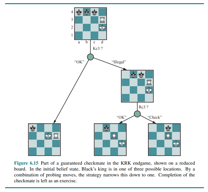
For Kriegspiel, a winning strategy, or guaranteed checkmate, is one that, for each possible percept sequence, leads to an actual checkmate for every possible board state in the current belief state, regardless of how the opponent moves. With this definition, the opponent’s belief state is irrelevant—the strategy has to work even if the opponent can see all the pieces.
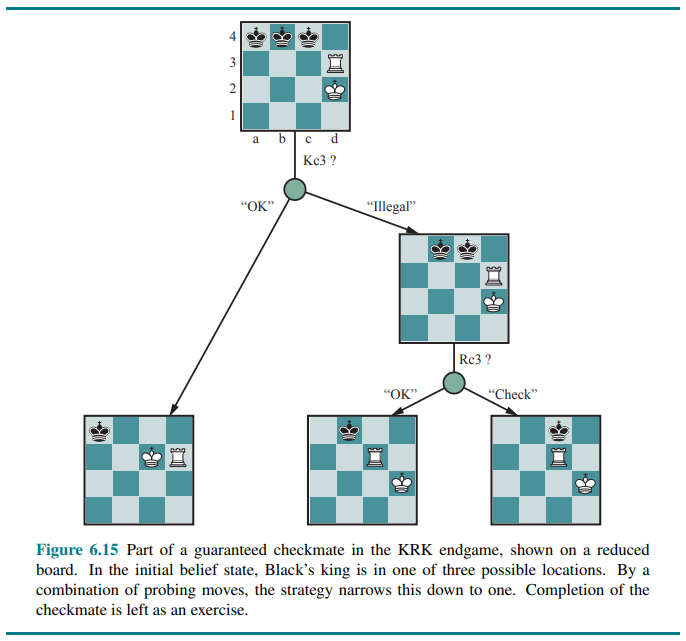 The general AND-OR search algorithm can be applied to the belief-state space to find guaranteed checkmates.
In addition to guaranteed checkmates, Kriegspiel admits an entirely new concept that makes no sense in fully observable games: probabilistic checkmate. Such checkmates are still required to work in every board state in the belief state; they are probabilistic with respect to randomization of the winning player’s move. To get the basic idea, consider the problem of finding a lone black king using just the white king. Simply by moving randomly, the white king will eventually bump into the black king even if the latter tries to avoid this fate, since Black cannot keep guessing the right evasive moves indefinitely. In the terminology of probability theory, detection occurs with probability 1.
The KBNK endgame—king, bishop and knight versus king—is won in this sense; White presents Black with an infinite random sequence of choices, for one of which Black will guess incorrectly and reveal his position, leading to checkmate. On the other hand, the KBBK endgame is won with probability
If Black happens to be in the right place and captures the bishop (a move that would be illegal if the bishops are protected), the game is drawn. White can choose to make the risky move at some randomly chosen point in the middle of a very long sequence, thus reducing
Sometimes a checkmate strategy works for some of the board states in the current belief state but not others. Trying such a strategy may succeed, leading to an accidental checkmate—accidental in the sense that White could not know that it would be checkmate—if Black’s pieces happen to be in the right places.
This idea leads naturally to the question of how likely it is that a given strategy will win, which leads in turn to the question of how likely it is that each board state in the current belief state is the true board state.
One’s first inclination might be to propose that all board states in the current belief state are equally likely—but this can’t be right. Consider, for example, White’s belief state after Black’s first move of the game. By definition (assuming that Black plays optimally), Black must have played an optimal move, so all board states resulting from suboptimal moves ought to be assigned zero probability.
This argument is not quite right either, because each player’s goal is not just to move pieces to the right squares but also to minimize the information that the opponent has about their location. Playing any predictable “optimal” strategy provides the opponent with information. Hence, optimal play in partially observable games requires a willingness to play somewhat randomly. (This is why restaurant hygiene inspectors do random inspection visits.)
This means occasionally selecting moves that may seem “intrinsically” weak—but they gain strength from their very unpredictability, because the opponent is unlikely to have prepared any defense against them.
From these considerations, it seems that the probabilities associated with the board states in the current belief state can only be calculated given an optimal randomized strategy; in turn, computing that strategy seems to require knowing the probabilities of the various states the board might be in. This conundrum can be resolved by adopting the game-theoretic notion of an equilibrium solution. An equilibrium specifies an optimal randomized strategy for each player. However computing equilibria is too expensive for Kriegspiel.
At present, the design of effective algorithms for general Kriegspiel play is an open research topic.
Most systems perform bounded-depth look-ahead in their own belief-state space, ignoring the opponent’s belief state. Evaluation functions resemble those for the observable game but include a component for the size of the belief state—smaller is better!
Card games
Card games such as bridge, whist, hearts, and poker feature stochastic partial observability, where the missing information is generated by the random dealing of cards.
At first sight, it might seem that these card games are just like dice games: the cards are dealt randomly and determine the moves available to each player, but all the “dice” are rolled at the beginning!
Even though this analogy turns out to be incorrect, it suggests an algorithm: treat the start of the game as a chance node with every possible deal as an outcome, and then use the EXPECTIMINIMAX formula to pick the best move.
Note that in this approach the only chance node is the root node; after that the game becomes fully observable.
This approach is sometimes called averaging over clairvoyance because it assumes that once the actual deal has occurred, the game becomes fully observable to both players. Despite its intuitive appeal, the strategy can lead one astray. Consider the following story:
- Day 1: Road A leads to a pot of gold; Road B leads to a fork. You can see that the left fork leads to two pots of gold, and the right fork leads to you being run over by a bus.
- Day 2: Road A leads to a pot of gold; Road B leads to a fork. You can see that the right fork leads to two pots of gold, and the left fork leads to you being run over by a bus
- Day 3: Road A leads to a pot of gold; Road B leads to a fork. You are told that one fork leads to two pots of gold, and one fork leads to you being run over by a bus. Unfortunately you don’t know which fork is which.
Averaging over clairvoyance leads to the following reasoning: on Day 1, B is the right choice; on Day 2, B is the right choice; on Day 3, the situation is the same as either Day 1 or Day 2, so B must still be the right choice.
Belief states and rational actions
- A naive idea is to define the value of an action as the average of its values across all possible hidden states (averaging over clairvoyance)
- In partially observable games, this intuition is wrong: the value of an action depends on the player’s information state or belief state.
- Therefore, optimal play must reason not only about world states, but also about how actions affect future information
- Key consequence: search can be performed over a tree of information states
- This leads to rational behaviours such as:
- acting to obtain information
- signalling to a partner
- randomizing to reduce information disclosure.
Now we can see how averaging over clairvoyance fails: it does not consider the belief state that the agent will be in after acting. A belief state of total ignorance is not desirable, especially when one possibility is certain death. Because it assumes that every future state will automatically be one of perfect knowledge, the clairvoyance approach never selects actions that gather information; nor will it choose actions that hide information from the opponent or provide information to a partner, because it assumes that they already know the information; and it will never bluff in poker.
Bluffing is good even when it’s not a core part of poker strategy.
Despite the drawbacks, averaging over clairvoyance can be an effective strategy, with some tricks to make it work better. In most card games, the number of possible deals is rather large.
For example, in bridge play, each player sees just two of the four hands; there are two unseen hands of 13 cards each, so the number of deals is
Another way to deal with the large number is forward pruning: consider only a small random sample of
So far we have assumed that each deal is equally likely. That makes sense for games like whist and hearts. But for bridge, play is preceded by a bidding phase in which each team indicates how many tricks it expects to win. Since players bid based on the cards they hold, the other players learn something about the probability
Taking this into account in deciding how to play the hand is tricky, for the reasons mentioned in our description of Kriegspiel: players may bid in such a way as to minimize the information conveyed to their opponents.
Computers have reached a superhuman level of performance in poker. The poker program Libratus took on four of the top poker players in the world in a 20-day match of no-limit Texas hold ’em and decisively beat them all. Since there are so many possible states in poker, Libratus uses abstraction to reduce the state space: it might consider the two hands AAA72 and AAA64 to be equivalent (they’re both “three aces and some low cards”), and it might consider a bet of 200 dollars to be the same as 201 dollars. But Libratus also monitors the other players, and if it detects they are exploiting an abstraction, it will do some additional computation overnight to plug that hole. Overall it used 25 million CPU hours on a supercomputer to pull off the win.
The computational costs incurred by Libratus (and similar costs by ALPHAZERO and other systems) suggests that world champion game play may not be achievable for researchers with limited budgets. To some extent that is true: just as you should not expect to be able to assemble a champion Formula One race car out of spare parts in your garage, there is an advantage to having access to supercomputers or specialty hardware such as Tensor Processing Units (TPUs).
For example the open-source LEELAZERO system is a reimplementation of ALPHAZERO that trains through self-play on the computers of volunteer participants.
ALPHASTAR won StarCraft II games running on a commodity desktop with a single GPU, and ALPHAZERO could have been run in that mode.
Limitations of Game Search Algorithms
Because calculating optimal decisions in complex games is intractable, all algorithms must make some assumptions and approximations.
Alpha–beta search uses the heuristic evaluation function as an approximation, and Monte Carlo search computes an approximate average over a random selection of playouts. The choice of which algorithm to use depends in part on the features of each game: when the branching factor is high or it is difficult to define an evaluation function, Monte Carlo search is preferred. But both algorithms suffer from fundamental limitations.
One limitation of alpha-beta search is its vulnerability to errors in the heuristic function:
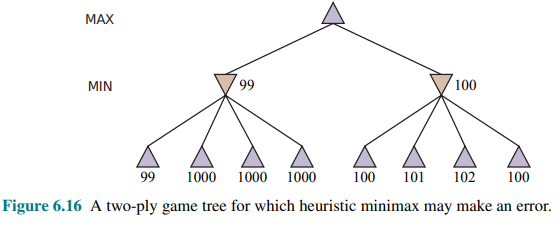
Figure 6.16 shows a two-ply game tree for which minimax suggests taking the right-hand branch because
If errors in the evaluation function are not independent, then the chance of a mistake rises. It is difficult to compensate for this because we don’t have a good model of the dependencies between the values of sibling nodes.
A second limitation of both alpha-beta and Monte Carlo is that they are designed to calculate (bounds on) the values of legal moves. But sometimes there is one move that is obviously best (for example when there is only one legal move), and in that case, there is no point wasting computation time to figure out the value of the move—it is better to just make the move.
A better search algorithm would use the idea of the utility of a node expansion, selecting node expansions of high utility—that is, ones that are likely to lead to the discovery of a significantly better move. If there are no node expansions whose utility is higher than their cost (in terms of time), then the algorithm should stop searching and make a move. This works not only for clear-favorite situations but also for the case of symmetrical moves, for which no amount of search will show that one move is better than another.
The kind of reasoning about what computations to do is called metareasoning (reason about reasoning). It applies not just to game playing but to any kind of reasoning at all. All computations are done in the service of trying to reach better decisions, all have costs, and all have some likelihood of resulting in a certain improvement in decision quality. Monte Carlo search does attempt to do metareasoning to allocate resources to the most important parts of the tree, but does not do so in an optimal way.
A third limitation is that both alpha-beta and Monte Carlo do all their reasoning at the level of individual moves. Clearly, humans play games differently: they can reason at a more abstract level, considering a higher-level goal. For example, trapping the opponent’s queen and using the goal to selectively generate plausible plans.
A fourth issue is the ability to incorporate machine learning into the game search process. Early game programs relied on human expertise to hand-craft evaluation functions, opening books, search strategies, and efficiency tricks. We are just beginning to see programs like ALPHAZERO which relied on machine learning from self-play rather than game-specific human-generated expertise.