AI - Lecture - Reasoning with uncertainty - Bayesian Networks

---

AI - Lecture - uncertainty Reasoning with Bayesian Networks

In real world agents have only partial knowledge of the world: incomplete information, noisy observations, unpredictable events and uncertain action outcomes.

Real-world problems contain uncertainties due to: partial observability, nondeterminism and adversaries. (See Environments and Adversarial Games)

For example: weather prediction, while current conditions provide evidence, tomorrow’s weather cannot be known with certainty.

Under uncertainty, an agent should reason with degrees of belief:

Why logic alone is not enough

Large domains such as medical diagnosis fail for three main reasons:

• Laziness: It is too much work to list the complete set of antecedents or consequents needed to ensure an exceptionless rule
• Theoretical ignorance: Medical science has no complete theory for the domain
• Practical ignorance: Even if we know all the rules, we might be uncertain about a particular patient because only some necessary tests have been or can be run

For example: dental diagnosis: .

• this logical rule is too strong: not every patient with a toothache has a cavity
• toothache may also be caused by gum disease, infection, trauma, etc.

We could try to make the rule logically exhaustive:

But this is impractical:

• the list of possible causes may be very large
• some causes may be unknown
• symptoms are not perfectly reliable.

Instead, probabilistic reasoning represents degrees of belief:

The idea is that a toothache does not logically imply a cavity but increases the probability of a cavity.

Acting under uncertainty

Real agents must act with incomplete and uncertain information. Probability theory allows agents to represent and update degrees of belief:

Decisions should consider both:

• how likely each outcome is
• how valuable or costly each outcome is

For example: a disease may be unlikely, but if the cost of missing it is high, the agent may still choose further testing.

Rational decision-making under uncertainty combines:

graph TD
    Uncertainty --> DoB

    subgraph Row1 [" "]
        direction LR
        DoB(Degree Of Belief) --> ProbabilityTheory(Probability Theory)
    end
    DoB --> PHYE("P(Hypothesis | Evidence)")
    
    subgraph Row2 [" "]
	    direction LR
	    PHYE -->|example| MedicalExample("$$P(Cavity \;| \;Toothache)$$")
    end

    style Row1 fill:none,stroke:none;
    style Row2 fill:none,stroke:none;

Probability

See:

• Probability, Sample Spaces and Events, Independent Event, Conditional Probability and Bayes Theorem (Statistics)
• Probability, Sample Spaces and Events, Independent Event, Conditional Probability and Bayes Theorem (Statistics)
• Bayesian Theory of Decision

Let’s make a recall there of these topics.

Uncertainty is represented by assigning probabilities to possible outcomes. A possible world is a complete description of one way the world could be.

The set of all possible worlds is called the sample space:

For example rolling a die we can get one of: . Each outcome corresponds to one possible world:

• die shows 1,
• die shows 2
• and so on

The probability of a world is written as . In the context of the fair die we know the outcome is:

Probability should satisfy some axioms:

• , in general 0 means impossible and 1 totally certain. We can draw a parallel with logic where we have only 0 or 1. Here we have values in between
• where is the set of all possible world.

An event is a set of possible worlds: For example the fair die:

For the event “roll an even number”:

Let’s consider another example: we roll two dices. This gives 36 equally likely possible worlds/outcomes:

Each outcome has a probability of .

if we care about the sum of the dice, there are 11 possible events:

Each sum value corresponds to an event i.e. a set of possible worlds. These events have different probabilities because some sums can be produced in more ways than others.

The probability of an event is:

Examples:

• because only produces 12
• because produce

Unconditional vs Conditional probability

Relevant note:

• The Bayesian Philosophy

Unconditional probability (Prior probability)

An unconditional probability, is a degree of belief in a proposition without considering any additional evidence.

In the previous die example:

Unconditional probability is also called prior probability.

Conditional probability

Represents belief in a proposition after observing evidence, defined as:

• : query/event of interest
• : observed evidence

This is an interesting definition because uses conjunction.

It represents how our belief in changes after learning that is true.

Intuition: once we know is true, we restrict attention to worlds where holds. Among these worlds, we ask how often is also true.

Equivalent to product rules:

Therefore, , this is the bayes rule.

Example conditional probability

For example consider two dices. The question is what is the probability that: i.e. probability to get a sum=12 given the first die draw is 6.

Start with 36 possible worlds:

Evidence is: .

We can restrict the sample space to worlds where the first die is 6: .

Among these 6 worlds, only one has sum 12:

Therefore:

We can write this using the formula:

Why ?

We have a conjunction so both terms should be true. Let’s reason in how many world you have that both occurs?

• is true in 1/36 because is equivalent to drawing a dice in a 2-fair-dice example
• can be true in every world e.g. imagine it is 1

Random variable

See:

• Random Variables

In probability theory, a random variable is a variable with a range of possible values it can take

• E.g., to represent the possible outcomes of rolling a die, we can define a random variable Roll that can take the values {1, 2, 3, 4, 5, 6}
• E.g., to represent the status of a flight, we can define a variable Flight that can take the values {on time, delayed, canceled}

We are interested in the probability with which each value occurs by using a probability distribution.

Consider this example:

Notation: a probability distribution can be represented as , to interpret this notation, the values have a set order, i.e., on time, delayed, canceled

We can introduce the concept of independence: two events and are independent if: in words knowing one doesn’t change the probability of the other. Also equivalentyl .

Example, rolling two dice:

The result of one die does not affect the result of the other.

Mathematically we can write: and are independent .

Dependent events are different: observing one event changes the probability of the other.

For example:

• If i observe in the morning some clouds, the probability that in the afternoon it will be raining is different of the probability of raining in the afternoon without any other information in the morning.

Bayes rule

• Bayes rule is very important in Bayesian Inference and therefore strongly used in machine learning

The bayes rule lets us update our belief in a hypothesis after observing evidence:

Terms:

• prior probability
• likelihood of the evidence if the hypothesis is true
• probability of the evidence
• posterior probability after observing evidence.

For example to infer: we can estimate the probabilities from observations i.e. collecting data:

Apply the Bayes’ rule:

Joint probability

Joint probability describes the probability that multiple events occur together:

For random variables, a joint distribution gives the probability of every combination of their values: , where for instance:

• =CloudyMorning =RainAfternoon

Marginal probabilities are not enough to know whether two variables are related e.g. and .

Using joint probabilities, we can deduce the conditional probability. In particular we need to look at the joint probabilities of all the possible outcomes of the two variables.

	R=rain	R=rain
C=cloud	0.08	0.32
C= cloud	0.02	0.58

Now we can know information about the co-occurrence of the events:

• For example, we know that the probability of a certain day having clouds in the morning and rain in the afternoon is 0.08
• The probability of no clouds in the morning and no rain in the afternoon is 0.58

Computing a conditional distribution from joint probability

We can compute: starting from the joint probabilities where we know that i.e. it will rain in the afternoon.

We see that:

These values are not yet a probability distribution over →

Normalize them so that they sum to 1:

• where called normalization factor

If we multiply by 0.08 and 0.02 we get thenormalized values.

Therefore:

The interpretation will be:

Visual

Consider previous table:

	R=rain	R=rain
C=cloud	0.08	0.32
C= cloud	0.02	0.58

If we consider it’s like restricting the table only to values present in this “query”, i.e. don’t consider the second column:

	R=rain
C=cloud	0.08
C= cloud	0.02

Probability rules

• Complement rule:
• Inclusion-exclusion rule:
  • intution: we count with the worlds where is true, and same with . Since worlds where both and are true are counted twice, we subtract once to correct the overlap.
  • Example:

Marginalization allows us to compute the probability of one event by summing over the possible cases of another event:

Intuition:

• when happens is either true or false
• the cases and are mutually exclusive
• together, they cover all possibilities.

For random variables:

• This means: to get the marginal probability of , sum the joint probabilities over all values of .

For example, from the joint table:

	R=rain	R=rain
C=cloud	0.08	0.32
C= cloud	0.02	0.58

To compute , sum over all possible values of :

• Replacing value from table:
• So

Probability rules: conditioning

• similar to marginalization

We can compute (unconditional probability) by conditioning on another event :

Intuition:

• either is true or is true
• these two cases are mutually exclusive
• together, they cover all possible worlds

So the probability of is a weighted average:

• probability of when is true
• probability of when is false

General form for random variable

This is called the rule of total probability

Example:

• Let the probability of raining be:

• Using previous values:

	R=rain	R=rain
C=cloud	0.08	0.32
C= cloud	0.02	0.58

• ,
• Then:

---

Bayesian networks

A Bayesian network represents uncertain knowledge using a graph structure and local condition probability distribution.

Syntax:

• one node for each random variable
• directed acyclic graph (DAG)
• edge is the parent of
• each node stores:

A bayesian network compactly represents a full joint probability distribution by exploiting conditional independence assumptions. We know that the joint probability is defined as:

(See also: NLP - Chain Rule for Words)

In Bayesian Network, the graph encodes conditional independence assumptions. Therefore, each variable only needs to be conditioned on its parents:

So, the full joint distribution factorizes as:

Hence, a Bayesian Network represents a large joint distribution compactly by storing only local conditional probability tables.

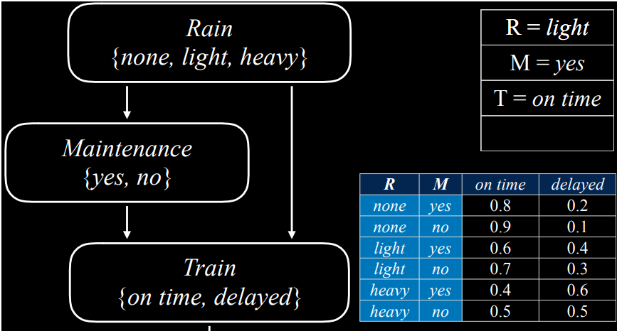
Example getting to an appointment on time

Consider the following:

graph TD
Rain("Rain<br>{none, light, heavy}")
Rain --> Maintenance("Maintenance<br>{yes,no}")
Maintenance --> Train("Train<br>{on time, delayed}")
Train --> Appointment("Appointment<br>{attend, miss}")
Rain --> Train

Rain is the root node:

• it has no parents, so it is described by a prior distribution
• It’s a random variable that can take the values with a probability distribution:

none	light	heavy
0.7	0.2	0.1

Maintenance encodes whether there is train truck maintenance, values () Its probability distribution is affected by Rain (Rain is its parent node):

R	yes	no
none	0.4	0.6
light	0.2	0.8
heavy	0.1	0.9

Train represents whether the train is on time or delayed, values (on time, delayed). It is affected by both Rain and Maintenace

R	M	on time	delayed
none	yes	0.8	0.2
none	no	0.9	0.1
light	yes	0.6	0.4
light	no	0.7	0.3
heavy	yes	0.4	0.6
heavy	no	0.5	0.5

Appointment represents whether one attends his appointment, values (attend, miss)

T	attend	miss
on time	0.9	0.1
delayed	0.6	0.4

Let’s consider a query

Query definition

Let be the complete set of the random variables in the bayesian network A query is a request to compute the conditional probability over a subset of these variables, given an assignment of values to another subset

Consider the following query as example; we want to compute the probability of this complete assignement:

From the Bayesian Network factorization:

Therefore:

• numerical values are obtained from all the previous tables.

Inference by enumeration

Probabilistic inference computes new beliefs from known probabilities. The result is usually a probability distribution, not a certain fact.

An inference query has three parts:

• Query variable : the variable whose probability distribution we want to compute
• Evidence variables : variables whose values have been observed
• Hidden variables : variables that are niether queried nor observed

Goal:

• where is the observed value of evidence variables.

Hidden variables are handled by summing over their possible values:

• where is a normalization constant (see prev example in this lesson)

graph TD
BN("Bayesian Networks")
BN --is a-->GraphStructure("Graph")
GraphStructure --> DAG
GraphStructure --> RandomVariable("each Node=X")
CIAssFormula("$$P(X_1,X_2,\dots, X_n) = \prod_{i=1}^n P(X_i|Parents(X_i))$$")
BN --Property--> CIAss("Conditional independence assumption") --Defined--> CIAssFormula
CIAssFormula --> Query
RandomVariable --> Query
Query --Example--> QueryExample("$$P(R=light,M=no,T=delayed,A=miss)$$")
QueryExample-->InferenceQuery("Inference Query")
InferenceQuery-->InferenceByEnumeration("Inference by enumeration")
InferenceByEnumeration--Goal-->PXE("$$P(X|E)$$")
InferenceByEnumeration--Hidden Variables-->HV("$$P(X|Y) = \alpha \sum_Y P(X,E,Y)$$")

Inference example

Query: Evidence is

Hidden variable:

Use marginalization over Train:

For maginalization see Probability rules and Probability rules conditioning

Then using Bayesian network factorization:

Result in:

• with order value

Bayesian Networks in Python

We can use the pomegranate library to implement Bayesian Networks.

Defining Nodes and Probabilities

First, we create the nodes and provide a probability distribution for each one.

from pomegranate import *
 
# Rain node has no parents
rain = Node(DiscreteDistribution({
    "none": 0.7,
    "light": 0.2,
    "heavy": 0.1
}), name="rain")
 
# Track maintenance node is conditional on rain
maintenance = Node(ConditionalProbabilityTable([
    ["none", "yes", 0.4],
    ["none", "no", 0.6],
    ["light", "yes", 0.2],
    ["light", "no", 0.8],
    ["heavy", "yes", 0.1],
    ["heavy", "no", 0.9]
], [rain.distribution]), name="maintenance")
 
# Train node is conditional on rain and maintenance
train = Node(ConditionalProbabilityTable([
    ["none", "yes", "on time", 0.8],
    ["none", "yes", "delayed", 0.2],
    ["none", "no", "on time", 0.9],
    ["none", "no", "delayed", 0.1],
    ["light", "yes", "on time", 0.6],
    ["light", "yes", "delayed", 0.4],
    ["light", "no", "on time", 0.7],
    ["light", "no", "delayed", 0.3],
    ["heavy", "yes", "on time", 0.4],
    ["heavy", "yes", "delayed", 0.6],
    ["heavy", "no", "on time", 0.5],
    ["heavy", "no", "delayed", 0.5],
], [rain.distribution, maintenance.distribution]), name="train")
 
# Appointment node is conditional on train
appointment = Node(ConditionalProbabilityTable([
    ["on time", "attend", 0.9],
    ["on time", "miss", 0.1],
    ["delayed", "attend", 0.6],
    ["delayed", "miss", 0.4]
], [train.distribution]), name="appointment")

Creating and Baking the Model

Second, we create the model by adding all the nodes and then describing which node is the parent of which other node by adding edges between them.

# Create a Bayesian Network and add states
model = BayesianNetwork()
model.add_states(rain, maintenance, train, appointment)
 
# Add edges connecting nodes
model.add_edge(rain, maintenance)
model.add_edge(rain, train)
model.add_edge(maintenance, train)
model.add_edge(train, appointment)
 
# Finalize model
model.bake()

Using the Model

For asking how probable a certain event is, we run the model with the values we are interested in.

# Calculate probability for a given observation
probability = model.probability([["none", "no", "on time", "attend"]])
print(probability)
 
# Calculate predictions based on evidence (e.g., train was delayed)
predictions = model.predict_proba({
    "train": "delayed"
})
 
# Print predictions for each node
for node, prediction in zip(model.states, predictions):
    if isinstance(prediction, str):
        print(f"{node.name}: {prediction}")
    else:
        print(f"{node.name}")
        for value, probability in prediction.parameters[0].items():
            print(f" {value}: {probability:.4f}")

Cons of Inference by Enumation

Inference by enumeration is an exact inference method. However, it can be computationally inefficient:

• it may require summing over all combinations of hidden variables
• the number of combinations grows exponentially with the number of variables

For many variables, exact inference may become impractical:

To handle large Bayesian networks, we often use approximate inference:

• faster computation
• some loss of precision
• accuracy improves with more samples

Sampling is a common approximate inference technique:

• Generate many random assignments according to the network probabilities
• Estimate probabilities from the frequency of outcomes

Sampling

Sampling estimates a probability distribution by generating many random outcomes.

Example: rolling a fair die

Suppose we roll the die 600 times

For each value, count how many times it appears

Estimate each probability by relative frequency:

For a fair die, the true probability is

so each value is expected to appear about times

The sampled distribution will probably not be exactly:

but it should be close

Approximate inference: sampling

Sampling estimates probabilities by generating many complete assignments of the network variables.

Variables are sampled in topological order:

Start with root node:

So:

• with probability
• with probability
• with probability

Approximate Inference: Forward Sampling

Suppose the first sampled value is: .

Next, we sample Maintenace.

Since rain is the parent of Maintenace, we use the conditional distribution:

Then

One full pass through the network generates one complete sample: .

An example sample: is:

Repeating the process many times produces a collection of samples. Then we estimate probabilities by counting frequencies :

Example:

As the number of samples increases, the estimate approaches the true probability

Approximate inference: Query

With query: , estimate the probability by counting samples:

Approximate Inference: Conditional Queries

Query:

With samples, estimate the conditional probability by filtering and counting.

1. Keep only samples consistent with the evidence so Train = on time
2. Among these samples, count how many also satisfy the query: Rain = light

Bayesian Networks in Python: Sampling

Approximate Inference via Sampling

from collections import Counter
 
def generate_sample():
    # Mapping of random variable name to sample generated
    sample = {}
    # Mapping of distribution to sample generated
    parents = {}
    # Loop over all states, assuming topological order
    for state in model.states:
        # If we have a non-root node, sample conditional on parents
        if isinstance(state.distribution, ConditionalProbabilityTable):
            sample[state.name] = state.distribution.sample(parent_values=parents)
        # Otherwise, just sample from the distribution alone
        else:
            sample[state.name] = state.distribution.sample()
        # Keep track of the sampled value in the parents mapping
        parents[state.distribution] = sample[state.name]
    # Return generated sample
    return sample
 
# Rejection sampling to compute P(Appointment | Train = delayed)
N = 10000
data = []
# Repeat sampling 10,000 times
for i in range(N):
    sample = generate_sample()
    # If, in this sample, the variable of Train has the value delayed, save it
    if sample["train"] == "delayed":
        data.append(sample["appointment"])
print(Counter(data))

To compute , which is the probability distribution of the Appointment variable given that the train is delayed:

# Rejection sampling
# Compute distribution of Appointment given that train is delayed
N = 10000
data = []
# Repeat sampling 10,000 times
for i in range(N):
	# Generate a sample based on the function that we defined earlier
	sample = generate_sample()
	# If, in this sample, the variable of Train has the value delayed, save it
	if sample["train"] == "delayed":
		data.append(sample["appointment"])
	# Count how many times each value of the variable appeared. We can later normalize
	print(Counter(data))

Alternative sampling methods

Whenever we want to ask the query conditional probability, the problem of sampling is: if the evidence is not so probable, we have just few examples that satisfy the evidence.

Too few example → not enough evidence → not good enough estimate

So having the sampling in the way we done, the risk is that we generate many many samples in order to have to satisfy the evidence. So let’s edit the sampling to adapt the query to conditional probability. In other words where the evidence is satisfied.

We consider two alternative sampling methods for probabilistic inference under uncertainty.

The first is rejection sampling: it generates complete samples of all variables in the Bayesian Network (e.g., Rain, Maintenance, Train, Appointment). It keeps only samples consistent with the evidence and reject all the other samples. The cons of this technique is that it is inefficient when the evidence is rare (e.g., Train = delayed rarely occurs), many generated samples may be discarded.

The other method is likelihood weighting

Likelihood weighting

Likelihood weighting:

• fix the evidence variables to their observed values,
• sample only the non-evidence variables
• assign each sample a weight based on how likely the evidence is:

Suppose we have a query

Evidence variable is: (enforcement)

Now we want to sample all the remaining variables (non-evidence variables): Rain, Maintenace and Appointment.

The approach is weight each sample by the probability of evidence:

The weight depends on the samples values of the parents of Train:

The cons of this approach is that: we enforced but it is not naturally generated according to this distribution.

Starting point:

graph TD
ConsOfInferenceByEnumeration("<small>Cons of Inference by Enumerations</small>")

ConsOfInferenceByEnumeration--Alternative-->ApproximateInference(Approximate Inference)-->Sampling

Sampling-->ForwardSampling("Forward Sampling")-->Query-->ConditionalQuery("Conditional Query")
Sampling-->AltSampMet("Alternative Sampling Methods")
AltSampMet-->RejectionSampling("Rejection Sampling")
AltSampMet-->LikeWeigh("Likelihood Weighting")

LikeWeigh-->FormulaLikeWeigh("$$w= \prod_{E_i \in Evidence} P(E_i = e_i | Parents(E_i))$$")-->ConsLikeWeigh("Cons of Likelihood Weighting")

Uncertainty

Many uncertain processes evolve over time:

• the weather today depends on the previous weather
• a robot’s position changes over itme
• a patient’s condition changes over time.

Let be the state of the world at time .

For example:

Without simplification, predicting may require the full history:

We can make the Markov assumption: The current state depends only on the previous state, not on the entire past.

Markov Assumption

See also

• Markov Chain, Markov Models, Hidden Markov Models (HMM)
• NLP - Language Models, N-Grams, Perplexity

A markov chain is a sequence of random variables where each variable satisfies the Markov assumption:

Markov Chain: Transition Model

A Markov chain describes how a state changes over time:

Under the Markov assumption:

Therefore, we only need a transition model:

The transition model specifies the probability of moving from one state to another.

Example Transition Model

For example:

	0.8	0.2
	0.4	0.6
A transition model tells us how beliefs evolve from one time step to the next.

Summary

• Real-world agents often act with incomplete and uncertain information
• Probability theory provides a formal language for representing degrees of belief
• Conditional probability allows beliefs to be updated when evidence is observed

• Bayes’ rule connects prior beliefs, evidence, and posterior beliefs

• Bayesian Networks represent joint probability distributions compactly

• Probabilistic inference computes query distributions given evidence
• Exact inference can be expensive, so approximate methods such as sampling are often used
• Temporal uncertainty can be modelled using Markov assumptions and transition models
• Probability allows AI agents to update their beliefs from evidence and make rational decisions under uncertainty