AI - Lecture - Solving Problems by Searching
- Source: Book Artificial Intelligence A Modern Approach 4 edition global edition - Russel - Chapter 3
Problem-solving agent and Search When the correct action to take is not immediately obvious, an agent may need to plan ahead: to consider a sequence of actions that form a path to a goal state. Such an agent is called a problem-solving agent, and the computational process it undertakes is called search.
Let’s first begin by considering the simplest environments: episodic, single agent, fully observable, deterministic, static, discrete and knwonw.
Informed vs uninformed algorithms: in informed algorithms the agent can estimate how far it is from the goal, whil in uniformed algorithms no such estimate is available.
Problem-Solving Agents
Example: an agent enjoying a touring vacation in Romania. The agent wants to take in the sights, improve its Romanina, enjoy the nightlife, avoid hangovers and so on (Goal). Suppose the agent is in the city of Arad and has a nonrefundable ticke to fly out of Bucharest the following day. The agent observes street signs and sees that there are three roads leading out of Arad: one toward Sibiu, one to Timisoara and one to Zerind. None of these are the goal, so unless the agent is familiar with the geography of Romania, it will not know which road to follow. Without additiona information (environment is unknown), then the agent can do no better than execute one of the actions at random.
If we give the agent information about the world for example this map:

Then the agnet can follow this four-phase problem-solving process:
- Goal Formulation: The agent adopts the goal of reaching Bucharest. Goals organize behavior by limiting the objectives and hence the actions to be considered.
- Problem formulation: The agent devises a description of the states and actions necessary to reach the goal—an abstract model of the relevant part of the world. For our agent, one good model is to consider the actions of traveling from one city to an adjacent city, and therefore the only fact about the state of the world that will change due to an action is the current city
- Search: Before taking any action in the real world, the agent simulates sequences of actions in its model, searching until it finds a sequence of actions that reaches the goal. Such a sequence is called a solution. The agent might have to simulate multiple sequences that do not reach the goal, but eventually it will find a solution (such as going from Arad to Sibiu to Fagaras to Bucharest), or it will find that no solution is possible.
- Execution: The agent can now execute the actions in the solution, one at a time
It is an important property that in a fully observable, deterministic, known environment, the solution to any problem is a fixed sequence of actions: drive to Sibiu, then Fagaras, then Bucharest.
Open vs closed loop systems: Control theorists calls an open-loop system a system where if the model is correct, it can ignore the percepts because following the fixed sequence of actions surely lead to a solution. Otherwise, if there is a chance that the model is incorrect, or the environment is nondeterministic, then the agent would be safer using a closed-loop approach that monitors the percepts.
Search problems and solutions
A search problem can be defined formally as follows:
- A set of possible states that the environment can be in. We call this the state space.
- The initial state that the agent starts in e.g. Arad
- A set of one or more goal states. Sometimes there is one goal state (e.g., Bucharest), sometimes there is a small set of alternative goal states, and sometimes the goal is defined by a property that applies to many states (potentially an infinite number).
- The actions available to the agent. Given a state
, returns a finite set of actions that can be executed in . We say that each of these actions is applicable in . An example: - A transition model, which describes what each action does.
returns the state that results from doing action in state . Fo rexample: . - Action cost function, denoted by ACTION-COST
when we are programming or when we are doing math, that ives the numeric cost of applying action in state to reach state . A problem-solving agent should use a cost function that reflects its own performance measure; for example, for route-finding agents, the cost of an action might be the length in miles or it might be the time it takes to complete the action.
Path: a sequence of actions from a path, and a solution is a path from the initial state to a goal state. We assume that action costs are additive; that is, the total cost of a path is the sum of the individual action costs. Optimal solution: is a solution that has the lowest path cost among all solutions.
The state space can be represented as a graph in which the vertices are states and the Graph directed edges between them are actions.
When formulating problems another important thing to consider are abstractions. Abstraction is the process of removing detail from a representation. A good problem formulation has the right level of detail. For instance if the actions were at the level of “Move the right foot forward a centimeter” the agent would probably never find its way out of the parking lot, let alone to Bucharest.
We can be more precise about the aprpopriate level of abstraction, like think of the abstract states and actions that we have chosen as corresponding to large sets of detailed world states and detailed action sequences. . Now consider a solution to the abstract problem: for example, the path from Arad to Sibiu to Rimnicu Vilcea to Pitesti to Bucharest. This abstract solution corresponds to a large number of more detailed paths. For example, we could drive with the radio on between Sibiu and Rimnicu Vilcea, and then switch it off for the rest of the trip.
The abstraction is:
- valid if we can elaborate any abstract solution into a solution in the more detailed world; a sufficient condition is that for every detailed state that is “in Arad,” there is a detailed path to some state that is “in Sibiu,” and so on.
- is useful if carrying out each of the actions in the solution is easier than the original problem; in our case, the action “drive from Arad to Sibiu” can be carried out without further search or planning by a driver with average skill.
Example Problems
Search algorithms are foundational to several critical domains where state-space exploration is required.
Navigation and Logistics
- Route Finding: Systems like GPS use Uniform-Cost Search (Dijkstra’s) to determine the minimum-cost path (distance or time) between geographical coordinates.
- Network Routing: Telecommunications protocols employ search algorithms to identify efficient paths for data packets across network nodes, minimizing latency and congestion.
Robotics and Motion Planning
- Pathfinding: Mobile robots utilize search to navigate from a starting configuration to a goal state while avoiding obstacles in a discretized environment.
- Assembly Sequences: In industrial manufacturing, search determines the sequence of operations required to assemble complex machinery without violating physical or spatial constraints.
Electronic Design Automation (EDA)
- VLSI Layout: The process of “routing” millions of wires between transistors on a microprocessor involves searching the physical layers of the chip to connect components without overlaps.
Combinatorial Optimization & Games
- Puzzle Solving: Classical problems such as the 8-puzzle or Rubik’s Cube are modeled as state-space search problems. Iterative Deepening is frequently used when the solution depth is unknown but memory is limited.
- Software Testing: Search-based engineering explores the execution state space of a program to identify paths leading to crashes or edge-case failures.
Scientific Research and Logic
- Chemical Synthesis: Planning a sequence of chemical reactions (actions) to synthesize a target molecule from precursors.
- Theorem Proving: Finding a logical proof for a mathematical conjecture by searching the state space of axioms and rules of inference. Breadth-First Search is often utilized to identify the shortest proof.
The Search Problem
A search algorithm takes a search problem as input and returns a solution, or an indication of Search algorithm failure.
The state-space is a graph, but for searching various algorithms and strategies superimose a search tree. Each node in the search tree corresponds to a state in the state space and the edges in the search tree correspond to actions.
State space vs search tree:
- The state space describes the (possibly infinite) set of states in the world, and the actions that allow transitions from one state to another.
- The search tree describes paths between these states, reaching towards the goal. It may have multiple paths to (and thus multiple nodes for) any given state, but each node in the tree has a unique path back to the root (as in all trees).
Best-First Search
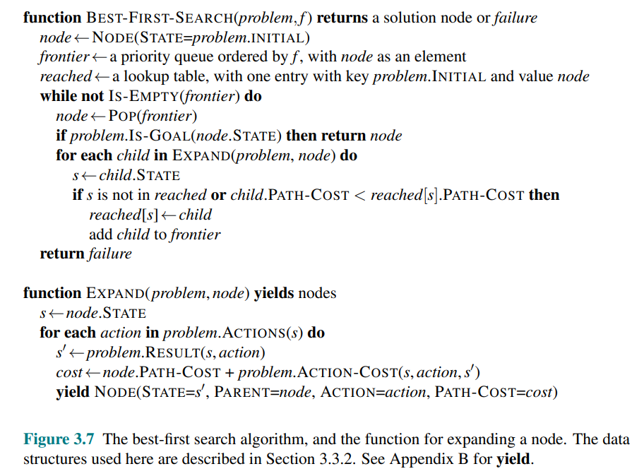
It is a general evaluation approach in which we choose a node
On each iteration we choose a node on the frontier with minimum
Redundant Paths

If we consider a path from Arad to Sibiu, you can go back to Arad, this is called a repeated state, that is generated by a cycle. Even though the state space has only 20 states, the complete search tree is infinite because there is no limit to how often one can traverse a loop. A cycle is a special case of a redundant path.
Measuring problem-solving performance
Evaluation metrics:
- Completeness: Is the algorithm guaranteed to find a solution when there is one, and to correctly report failure when there is not?
- Cost optimality: Does it find a solution with the lowest path cost of all solutions?
- Time complexity: How long does it take to find a solution?
- Space complexity: How much memory is needed to perform the search?
To be complete, a search algorithm must be systematic in the way it explores an infinite state space, making sure it can eventually reach any state that is connected to the initial state.
In theory, the thypical measure of the size of the state-space since we have a graph is
Uninformed Search Strategies
An uninformed search algorithm is given no clue about how close a state is to the goal(s).
For example, consider the agent in Arad, with the goal to reach Bucharest. If it is “uninformed” i.e. it doesn’t know the geography of Romany, then it has no clue of whetever going to Zerind or Sibiu is a better first step.
Main strategies:
- Breadth-first
- Depth-first
- Uniform-cost
- Depth-limited
- Iterative-deepening depth-first
- Bidirectional search
Breadth-first search (BFS)
When all actions have the same cost, an appropriate strategy is breadth-first search, in which the root node is expanded first, then all the successors of the root node are expanded next, then their successors, and so on.
It uses a FIFO query that gives the correct order of nodes. New nodes (which are always deeper than their parents) go to the back of the queue, and old nodes, which are shallower than the new nodes, get expanded first.
We can do an early goal test because we can check wheter a node is a solution as soon as it is generated i.e added to the FIFO.
Breadth-first search always finds a solution with a minimal number of actions, because when it is generating nodes at depth
If the solution is at depth
All nodes remains in memory so both space and computational complexity are
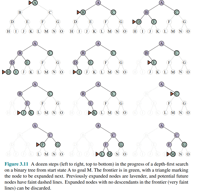
Depth-first search (DFS) and the problem of memory
Depth-first search always expands the deepest node in the frontier first. It is implemented as a tree-like search that does not keep a table of reached states.
The cost is:
is the branching factor, is the maximum depth of tree
It is not optimal even though it has low memory usage. If the graph has cycles it can get stuck in infinite loops, therefore some implementation that check for this is required. However, for problems where a tree-like search is feasible, depth-first search has much smaller needs for memory.
A variant of depth-first search called backtracking search uses even less memory. In backtracking, only one successor is generated at a time rather than all successors; each partially expanded node remembers which successor to generate next. In addition, successors are generated by modifying the current state description directly rather than allocating memory for a brand-new state.
Dijkstra’s algorithm or uniform-cost search
When actions have different costs, an obvious choice is to use best-first search where the evaluation function is the cost of the path from the root to the current node. This is called Dijkstra’s algorithm also called uniform-cost search.

Choose the path with the lowest cost i.e in meters. Starting from Bucharest, it find that Sibiu+Rimnicu Vilcea+ Pitesti + Bucharest is the shortest path. However, the algorithm tests for goals only when it expands a node, not when it generates a node, so it has not yet detected that this is a path to the goal.
The algorithm continues on, choosing Pitesti for expansion next and adding a second path to Bucharest with cost 80 + 97 + 101=278. It has a lower cost, so it replaces the previous path in reached and is added to the frontier. It turns out this node now has the lowest cost, so it is considered next, found to be a goal, and returned.
The complexity of uniform-cost search is characterized in terms of
The worst-case cost is
Depth-limited and iterative deepening search
To keep depth-first search from wandering down an infinite path, we can use depth-limited search. This version require that we supply a limit
The time complexity is
This algorithm find a solution only if we make a good choice of
Sometimes a good depth limit can be chosen based on knowledge of the problem. For example, on the map of Romania there are 20 cities. Therefore,
Iterative deepening search: solves the problem of picking a good value for by trying search all values: first 0, then 1, then 2, and so on—until either a solution is found, or the depthlimited search returns the failure value rather than the cutoff value.
Like depth-first search, its memory requirements are modest:
The time complexity is
It may seem a waste of resources but for many state spaces, most of the nodes are in the bottom level, so it does not matter much that the upper levels are repeated.
In the worst case, we have
Iterative Deepening Search combines advantages of DFS and BFS:
- like DFS it requires only linear space
- like BFS it is complete for finite branching factor
- it is optimal when all step costs are equal
In general, iterative deepening is the preferred uninformed search method when the search state space is larger than can fit in memory and the depth of the solution is not known.
Bidirectional search
The algorithms we have covered so far start at an initial state and can reach any one of multiple possible goal states.
An alternative approach called bidirectional search simultaneously searches forward from the initial state and backwards from the goal state(s), hoping tha the two searches meet.
The worst case cost would be
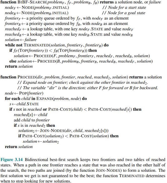
- Keep track of two frontiers and two tables of reached states
- when a solution is find then the two frontiers collide.
is the forward direction and is the backward direction - When the evaluation function is the path cost, we know that the first solution found will be an optimal solution, but with different evaluation functions that is not necessarily true.
Backward search requires:
- reversible actions, or
- hash table to check efficiently if two paths meet (i.e efficiently computable predecessor function)
Comparing uninformed search algorithms
| Criterion | Breadth-first | Uniform-cost | Depth-first | Depth-limited | Iterative deepening | Bidirectional |
|---|---|---|---|---|---|---|
| Completeness | Yes (if | Yes (if costs | No | No | Yes (if | Yes (if |
| Cost optimality | Yes (if same cost) | Yes | No | No | Yes (if same cost) | Yes (if same cost) |
| Time complexity | ||||||
| Space complexity |
is the branching factor, the maximum depth of the search tree, is the depth of the shallowest solution
Effectiveness of Uninformed Search
One migh expect uninformed search can be problematic only in large real-world problems. In fact, even a simple toy problems such as the 8-puzzle can make uninformed search computationally expensive.
Consider the 8-puzzle, an apparently simple problem. The 8-puzzle contains
It can be shown that the average solution depth (over all possible paris of initial and goal states is about 22.
The average branching factor
How many nodes does BFS generate and store when the shallowest solution has depth
This motivates the need for other kind of strategies, that are explored in the lecture: AI - Lecture - Solving Problems by Searching - Heuristic Search Strategies and Heuristic Functions