---

AI - Lecture Solving Problems by Searching - Search in Complex Environments §

• Source: Book Artificial Intelligence A Modern Approach 4 edition global edition - Russel - Chapter 4

We previously saw how search is addressed in fully observable, deterministic, static, known environments where the solution is a sequence of actions. In this chapter we relax those constraints.

Local Search and Optimization Problem §

Sometimes we care only about the final state, not the path to get there.

For example in the 8-queens problem: 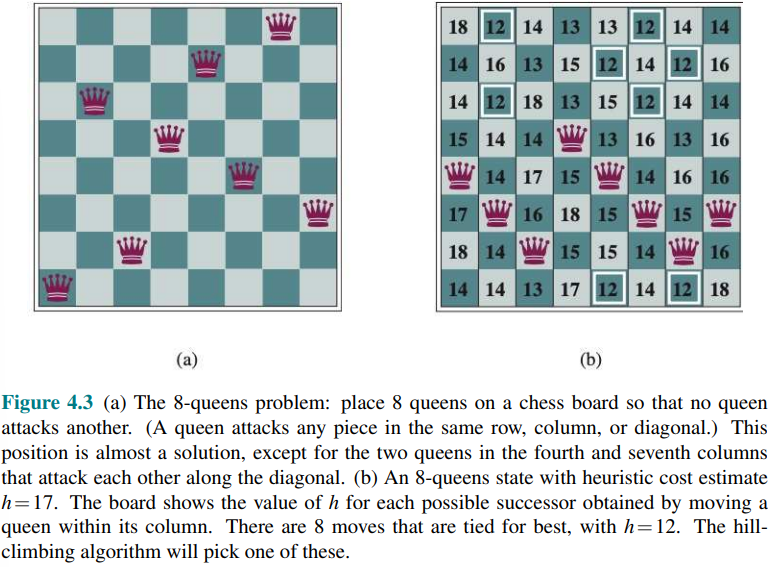we only care about findining a valid final configuration of 8 queens.

This is true also for many important applications such as integrated-circuit design, factory floor layout, job shop scheduling, automatic programming, telecommunications network optimization, crop planning and portfolio management.

Local search algorithms operate by searching from a start state to neighboring states, without keeping track of the paths, nor the set of states that have been reached. These algorithms are not systemic they might never explore a portion of the search space where a solution actually resides.

Local search algorithms have two advantages:

• They use very little memory
• They can often find a reasonable solutions in large or infinite state space for which systematic algorithms are unsuitable.

Local search algorithms can also solve optimization problems in which the aim is to find the best state according to an objective function (i.e. machine/deep learning).

Hill-Climbing Search §

• Also called greedy local search

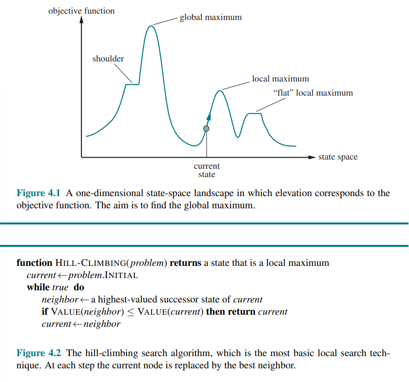
It keep track of one current state and on each iteration moves to the neighboring state with the highest value (it heads in the direction that provides the steepest ascent).

To illustrate hill climbing we can use the 8-queens problem: and we consider a complete-state formulation, which means that every state has all the components of a solution, but they might not all be in the right place.

The initial state is chosen at random, and the successors of a state are all possible states generated by moving a single queen to another square in the same column (so each state has successors). The heuristic cost function is the number of pairs of queens that are attacking each other; this will be zero only for solutions.

Unfortunately hill climbing (i.e. greedy local search) can get stuck for any of these following reasons:

• Local maxima: A local maximum is a peak that is higher than each of its neighboring states but lower than the global maximum. Hill-climbing algorithms that reach the vicinity of a local maximum will be drawn upward toward the peak but will then be stuck with nowhere else to go.
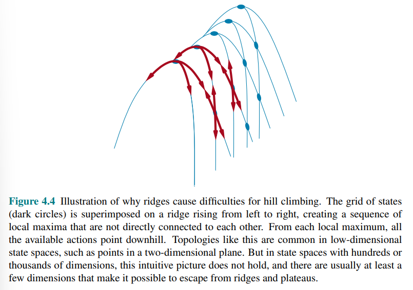
• Ridges: result in a sequence of local max that is very difficult for greedy algorithms to navigate
• Plateaus: is a flat area of the state-space landscape. It can be a flat local maximum, from which no uphill exit exists, or a shoulder from which progress is possible.

For the 8-queens state, the steepest-ascent hill climbing gets stuck 86% of the time, solving only 14% of problem instances. On the other hand, it works quickly.

To solve more problem, one answer is to keep going when we reach a plateau to allows a sideways move in the hope that the plateau is really a shoulder.

Many variant of hill climbing has been invented:

• Stochastic hill climbing chooses at random from among the uphill moves
• First-choice hill climbing implements stochastic hill climbing by generating successors randomly untile one is generated that is better than the current state
• Random-restart hill climbing: if at first it doesn’t suceed, it try again. It conducts a series of hill-climbing searches from randomly generated initial states, until a goal is found.

For the random restart hill climbing consider the following: if each hill-climbing search has a probability p of success, then the expected number of restarts required is . For 8 queens we have so we need roughly 7 iterations to find a goal (6 failures and 1 success). The expected number of steps is the cost of one successful iteration plus times the cost of failure, or roughly 22 steps in all. We we allow sideways moves, iterations are needed on average and steps. For 8-queen, then, random-restart hill climbing is very effective. Even for three million queens, the approach can find solutions in seconds.

The success of hill climbing depends very much on the shape of the state-space landscape: if there are few local maxima and plateaus, random-restart hill climbing will find a good solution very quickly

Simulated Annealing §

A hill-climbing algorithm that never makes “downhill” moves toward states with lower value (or higher cost) is always vulnerable to getting stuck in a local maximum.

Simulated annealing try to combine hill climbing with a random walk in a way that yields both efficiency and completeness.

Consider instead of hill climbing, the problem of finding local minimum i.e. gradient descent and imagine the task of getting a ping-pong ball into the deepest crevice in a very bumpy surface:

• If we just let the ball roll, it will come to rest at a local minimum.
• If we shake the surface, we can bounce the ball out of the local minimum—perhaps into a deeper local minimum, where it will spend more time.

The trick is to shake just hard enough to bounce the ball out of local minima but not hard enough to dislodge it from the global minimum. The simulated-annealing solution is to start by shaking hard (i.e., at a high temperature) and then gradually reduce the intensity of the shaking (i.e., lower the temperature).

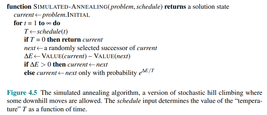
• It is very similar to hill climbing, however instead of picking the best move, it picks a random move.
• If the random move improves the situation, it is always accepted. Otherwise, the algorithm accepts the move with some probability less than 1.

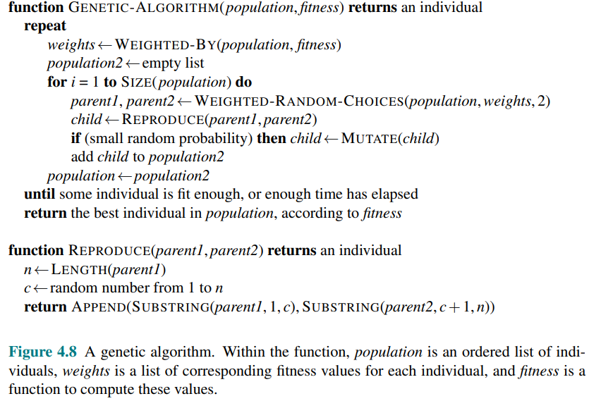
Evolutionary Algorithms §

Evolutionary algorithms are based on natural selection in biology: there is a population of individuals (states), in which the fittest (highest value) individuals produce offspring (successor states) that populate the next generation, a process called recombination.

There are endless forms of evolutionary algorithms, varying in the following ways.

• Size of the population
• Representation of each individual: e.g. in genetic algorithms an individual is often a Boolean string like DNA string over a finite alphabet like ACGT. In evolution strategies, an individual is a sequence of real numbers, and in genetic programming an individual is a computer program
• The mixing number which is the number of parents that come together to form offspring, the most common is where two parents combine their “genes” (parts of their representation) to form offspring. When we have stochastic beam search and occurs rarely but is easy enough to simulate
• The selection process for selecting which individuals become parents of the next generation. One possibility is select from all individuals with probability proportional to their fitness score. Another possibility is to randomly select n individuals () and then select the most fit ones as parents
• The recombination procedure: one common approach assuming is to randomly select a crossover point to split each of the parent strings, and recombine the parts to form two children, one with the first part of parent 1 and the second part of parent 2; the other with the second part of parent 1 and the first part of parent 2.
• The mutation rate, which determines how often offspring have random mutations to their representation. Once an offspring has been generated, every bit in its composition is flipped with probability equal to the mutation rate.
• The makeup of the next generation: this can be just newly formed offspring or it can include a few top-scoring parents from previous generation (practice called elitism, which guarantees that overall fitness will never decrease over time). . The practice of culling, in which all individuals below a given threshold are discarded, can lead to a speedup

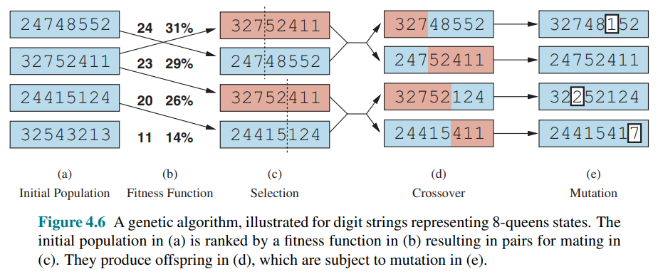
• 4.6 (a) shows the initial state of four 8-digit strings, each representing a state of the 8-queens puzzle, where the th digit represents the row number of the queen in column .
• 4.6(b) shows each state rated by the fitness function, in the case of this puzzle, the number of nonattacking queens which has a value of for a solution. The fitness scores are then normalized to probabilities
• In (c), two pairs of parents are selected, in accordance with the probabilities in (b). Notice that one individual is selected twice and one not at all.
• For each selected pair, a crossover point (dotted line) is chosen randomly
• In (d), we cross over the parent strings at the crossover points, yielding new offspring.
• Finally, in (e), each location in each string is subject to random mutation with a small independent probability. One digit was mutated in the first, third, and fourth offspring. In the 8-queens problem, this corresponds to choosing a queen at random and moving it to a random square in its column

Local Search in Continuous Spaces §

In previous lectures we explained the distinction between discrete and continuous environments, pointing out that most real-world environments are continuous.

A continuous action space has an infinite branching factor, and thus can’t be handled by most of the algorithms we have covered so far.

We find uses for these techniques in several places in this book, including the chapters on learning, vision, and robotics.

We begin with an example. Suppose we want to place three new airports anywhere in Romania, such that the sum of squared straight-line distances from each city on the map to its nearest airport is minimized.

The state space is then defined by the coordinates of the three airports: and . This is a six-dimensional space i.e. with six variables. In general, states are defined by an -dimensional vector of variables, .

Moving around in this space corresponds to moving one or more of the airports on the map.

The objective function is easy to compute for any particular state once we compute the closest cities: is relatively easy to compute for any particular state once we compute the closest cities.

Let be the set of cities whose closest airport (in the state x) is airport , we have:

This equation is correct not only for the state x but also for states in the local neighborhood of x. However, it is not correct globally; if we stray too far from (by altering the location of one or more of the airports by a large amount) then the set of closest cities for that airport changes, and we need to recompute .

One way to deal with a continuous state space is to discretize it. For example, instead of allowing the locations to be any point in continuous two-dimensional space, we could limit them to fixed points on a rectangular grid with spacing of size (delta). Then instead of having an infinite number of successors, each state in the space would have only 12 successors, corresponding to incrementing one of the 6 variables by . We can then apply any of our local search algorithms to this discrete space. Alternatively, we could make the branching factor finite by sampling successor states randomly, moving in a random direction by a small amount, .

Methods that measure progress by the change in the value of the objective function between two nearby points are called empirical gradient methods. Empirical gradient search is the same as steepest-ascent hill climbing in a discretized version of the state space.

Often we have an objective function expressed in a mathematical form such that we can use calculus to solve the problem analytically rather than empirically. Many methods attempts to use the gradient of the landscape to find a maximum. The gradient of the objective function is a vector that gives the magnitude and direction of the steepest slope.

For our problem, we have:

In some cases, we can find a maximum by solving the equation . This could be done, for example, if we were placing just one airport; the solution is the arithmetic mean of all the cities’ coordinates.

In many cases however this equation cannot be solved in a closed form.

For example consider with three airports, the expression for the gradient depends on what cities are closest to each airport in the current state. This means we can compute the gradient locally but not globally, for example:

Given a locally correct expression for the gradient, we can perform steepest-ascent hill climbing by updating the current state according to the formula:

where is the step size (also called learning rate in machine learning). A too small step size requires too many steps, while a too big step size overshoot the maximum.

For many problems, the most effective algorithm is the venerable Newton–Raphson method. It is the general technique for finding roots of functions. It works by computing a new estimate for the root according to Newton’s formula:

To find a maximum or minimum of , we need to find such that the gradient is a zero vector (i.e., ). Thus in Newton’s formula becomes , and the update equation can be written in matrix–vector form as:

• is the Hessian matrix of second derivatives whose element

For our airport example, we can see from Equation (4.2) that is particularly simple: the off-diagonal elements are zero and the diagonal elements for airport i are just twice the number of cities in . A moment’s calculation shows that one step of the update moves airport directly to the centroid of which is the minimum of the local expression for from Equation: .

For high-dimensional problems, however, computing the entries of the Hessian and inverting it may be expensive, so many approximate versions of the Newton–Raphson method have been developed.

Local search methods suffer from local maxima, ridges, and plateaus in continuous state spaces just as much as in discrete spaces. Random restarts and simulated annealing are often helpful. High-dimensional continuous spaces are, however, big places in which it is very easy to get lost.

A final topic is constrained optimization i.e. solutions must satisfy some hard constraints on the values of the variables. For example, in our airport-siting problem, we might constrain sites to be inside Romania and on dry land (rather than in the middle of lakes).

The best-known category is that of linear programming problems, in which constraints must be linear inequalities forming a convex set and the objective function is also linear. Linear programming is a special case of the more general problem of convex optimization which allows the constraint region to be any convex region and the objective to be any function that is convex within the constraint region.

Search with Nondeterministic Action §

In previous lessons we assumed a fully observable, deterministic, known environment. Therefore, an agent can observe the initial state, calculate a sequence of actions that reach the goal, and execute the actions with its “eyes closed,” never having to use its percepts.

However when the environment is partially observable, however, the agent doesn’t know for sure what state it is in. When the environment is nondeterministic, the agent doesn’t know what state it transitions to after taking an action.

That means that rather than thinking “I’m in state and if I do action a I’ll end up in state ,” an agent will now e thnking “I’m either in state or and if I do action a I’ll end up in state , or .”

Conditional Plan and Belief State: We call a set of physical state that the agent believes are possible a belief state. In partially observable and nondeterministic environments, the solution to a problem is no longer a sequence, but rather a conditional plan (sometimes called a contingency plan or a strategy) that specifies what to do depending on what percepts agent receives while executing the plan.

The erratic vacuum world §

Consider the vacuum world from previous example, with eight states and three actions: right, left, and suck, and the goal is to clean up all the dirt (states 7 and 8).

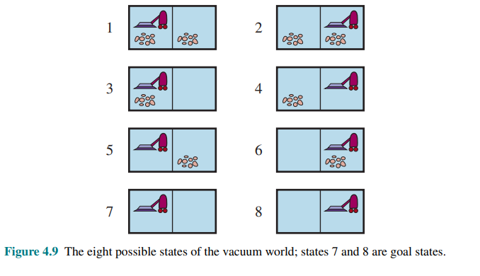
Now consider that we introduce nondeterminism in this world. In the erratic vacuum world the Suck action works as follows:

• When applied to a dirty square the action cleans the square and sometimes cleans up dirt in an adjacent square, too
• When applied to a clean square the action sometimes deposits dirt on the carpet.

To provide a precise formulation of this problem, we need to generalize the notion of a transition model; instead of deiniing the transition model by a RESULT function that returns a single outcome state, we use a RESULTS function that returns a set of possible outcome states.

For example, in the erratic vacuum world, the Suck action in state 1 cleans up either just the current location, or both locations:

If we start in state 1, no single sequence of actions solves the problem, but the following conditional plan does:

Here we see that a conditional plan can contain if–then–else steps; this means that solutions are trees rather than sequences. Here the conditional in the if statement tests to see what the current state is; this is something the agent will be able to observe at runtime, but doesn’t know at planning time. Alternatively, we could have had a formulation that tests the percept rather than the state.

Many problems in the real, physical world are contingency problems, because exact prediction of the future is impossible.

AND-OR search trees §

How do we find these contingent solutions to nondeterministic problems? We begin by constructing search trees, but here the trees have a different character. We have two kind of nodes:

• OR Nodes: an agent can do this action or that action. In the vacuum world for example, at an OR node the agent chooses Left or Right or Suck.
• AND Nodes: for example the Suck action in state 1 results in the belief state so the agent would need to find a plan for state 5 and for state 7

These kinds of nodes alternate, leading to an AND-OR tree:

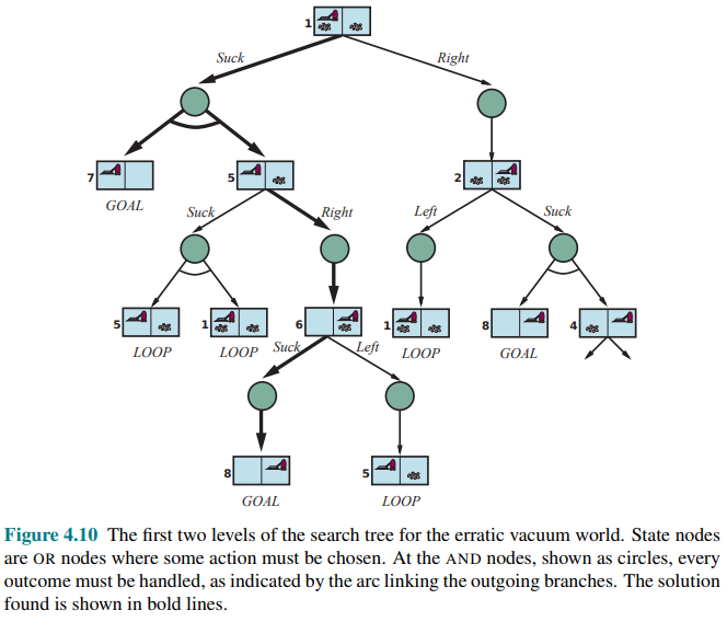
A solution for an AND-OR search problem is a subtree of the complete search tree that:

1. Has a goal node at every leaf
2. Specifies one action at each of its OR nodes
3. Includes every outcome branch at each of its AND nodes.

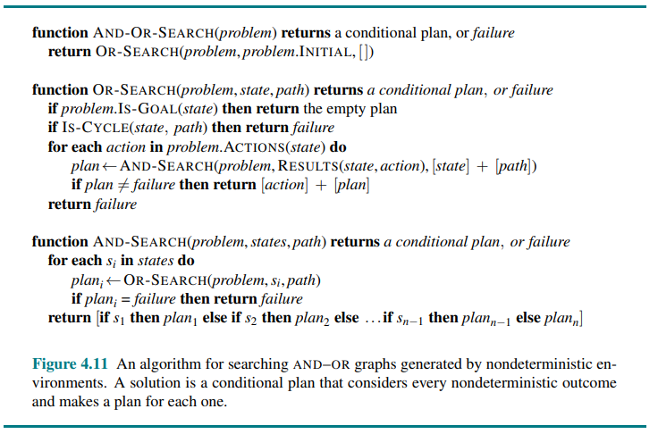
If the current state is identical to a state on the path from the root, then it returns with failure. This doesn’t mean that there is no solution from the current state; it simply means that if there is a noncyclic solution, it must be reachable from the earlier incarnation of the current state, so the new incarnation can be discarded. With this check, we ensure that the algorithm terminates in every finite state space, because every path must reach a goal, a dead end, or a repeated state.

Notice that the algorithm does not check whether the current state is a repetition of a state on some other path from the root, which is important for efficiency.

Try, try again §

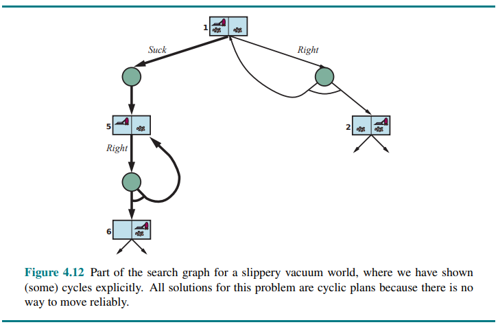
Consider a slippery vacuum world. which is identical to the ordinary (non-erratic) vacuum world except that movement actions sometimes fail, leaving the agent in the same location.

For example, moving Right in state 1 leads to their belief state :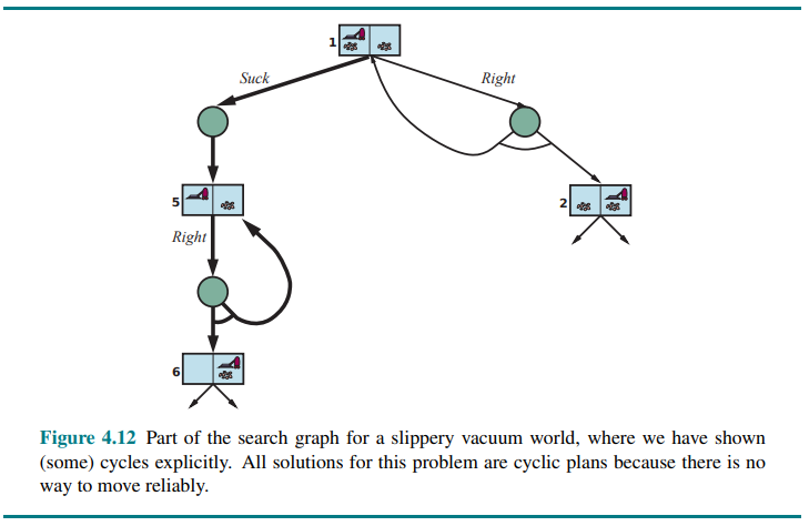

Figure 4.12 shows part of the search graph; clearly there are no longer any acyclic solutions from state 1, and AND-OR-SEARCH would return with failure. There is, however, a cyclic solution, which is to keep trying Right until it works.

We can express this with a new while construct:

or by adding a label to denote some portion of the plan and referring to that label later:

When is a cyclic plan a solution? A minimum condition is that every leaf is a goal state and that a leaf is reachable from every point in the plan. In addition to that, we need to consider the cause of the nondeterminism.

But if the nondeterminism is due to some unobserved fact about the robot or environment—perhaps a drive belt has snapped and the robot will never move—then repeating the action will not help.

One way to understand this decision is to say that the initial problem formulation (fully observable, nondeterministic) is abandoned in favor of a different formulation (partially observable, deterministic) where the failure of the cyclic plan is attributed to an unobserved property of the drive belt.