SC - Lezione 12 - SVD Application for Latent Semantic Analysis and Principal Component Analysis (PCA)

---

SC - Lezione 12 §

---

Checklist §

Checklist

Domande, Keyword e Vocabulary §

• SVD Applications
• SVD in Latent Semantic Analysis
• query in semantic analysis
• cosine similarity
• data dimensionality reduction
• SVD and image compression
• SVD e Principal Component Analysis
• PCA Introduction in statistics
• Principal Components
• Application of the SVD on PCA
• Anomaly Matrix
• Covariance Matrix
• Dominants eigenvalue and eigenvector
• PCA in statistics
• PCA and Spectral Decomposition
• SVD and PCA Application: Eigenfaces

Appunti SC - Lezione 12 §

SVD in Latent Semantic Analysis §

We did the same with the QR applications.

This problem isn’t anymore a semantic problem but a linear algebra problem.

Consider documents of length n and terms of length m. We obtain a matrix terms-documents in (notice the matrix is non square)

The first column corresponds to the first documents and it is read as contains these word (1 contains the term, 0 doesn’t contains the term).

The columns of this matrix have size and the rows have size . The matrix can be interpretated in this way: for example in the third column we have the third document that is “Automatic differentiation of algorithms: theory, implementation and application” in which appears the terms “algorithms”, “application”, “implementation” and “theory”.

So we have the features on the columns and the data on the rows.

When we do semantic analysis we are interested into satisfying a query. A query will be a vector with as many component as a column () that satisfy a logical expression like “find the documents that contains ‘applications’ and ‘theory’“.

We will use the cosine similarity that we already know:

Data Dimensionality Reduction: The idea is that i don’t want to work on a 16-dimension space, but i want to work in a reduced dimension space by projecting both terms and document onto a subspace of smaller dimension.

We use the SVD factorization of the matrix B:

The SVD factorization allows us to project both the row subspace and column subspace into a smaller subspace. For the similarity of the query i’m forced to consider the column subspace.

In order to apply the dimension reduction to we want to consider the rank-k approximation:

Where:

• The columns of forms an orthonormal basis of a subspace of dimension of the column space of
• The rows of forms an orthonormal basis of a subspace of dimension of the row space of

In general, the -th document is approximated by the -th column of whose components in the basis are the components of column in

In the matlab example we represented the documents in the space of dimension k=2 just for showing on a plane, otherwise for k=4 we cannot represent it.

Both and are orthogonal with respect to the columns. In the example i consider the subspace of dimension 2 in which i’m representing the documents and this space is generated by the two columns of . So i project my query into this subspace and for doing this i apply the following: (,q hat,)

SVD and image compression §

Let’s consider a gray-level image. An image is a matrix composed of pixels. We approximate this matrix by means of the k-truncated SVD We can write that:

• where

The interesting idea is to see the factorization as a sum of matrices of rank 1 with less information. Each image added to the previous one add more information. And in practice the image becomes more nitid and more details are shown. We still get a good enough approximation if we don’t consider the maximum k.

In the following example we see an image with colors. That is simply three matrices one for Red, one for Green and one for Blue values.

To check the “error” (that is ) we use the frobenius norm. In the graph of the frobenius norm we notice that, as we expect, the more you use, the more the error decreases.

Riga codice:

AErrFinal = cat(3,uint8(AerrR),uint8(AerrG),uint8(AerrB));

cat mette le matrici una sopra l’altra come se fossero dei piatti.

SVD and Principal Component Analysis §

PCA definition in short §

PCA is an orthogonal linear transformation of the data that maps the data into a new reference system in order to maximize the variance (with respect to any other orthogonal reference system) associated with the first coordinate (first principal component), and then that associated with the second coordinate (second principal component), and so on.

PCA - Principal Component Analysis §

Consider a set of data, the data matrix in which the features are placed on the columns, while the measurements for each experiment are placed on the rows.

Let us consider an example with characteristics height and weight of a person. In this case, the data is arranged in such a way that we need to look at the row space, i.e the columns of the matrix ().

PCA introduction in statistics §

Before diving into this, however, let’s introduce PCA (Principal Component Analysis) as it is used in statistics.

Suppose that data in my dataset lie along a straight line.

We can compute:

• The mean, which provides the central value, representing the most typical or representative point of the dataset.
• The variance (or equivalently, the square of the standard deviation), which measures how spread out the data is.

Let’s assume that data is two-dimensional, meaning the points lie on a plane. If you look on the x-coordnates there will be a minimum and maximum value. The variability of the x-coordinates is the spread between these values.

Similarly, we can observe the spread in the y-coordinates by looking at their minimum and maximum values. We can say that the variance along the first axis is given by the y-values and the variance across the second axis is given by the x-values.

Now consider that you change the reference system by rotating the data matrix. After that you have to apply the orthogonal projection onto the new basis. If we compute again the spread across the new x-axes and y-axes, we notice that will be different.

Principal Component Analysis (PCA) helps identify the optimal rotation of the data, providing a new orthogonal coordinate system that maximizes the variance along the first axis. Specifically, PCA seeks the rotation where the variance along the first axis (the first principal component) is maximized. The remaining variance is then maximized along the second axis (the second principal component), and so on.

The axes of this new orthogonal system are called the principal components, and the first principal component is the one along the axis where the variance is maximized. Similarly, the second principal component is the one where the remaining variance is maximized, and so on for the third, fourth, etc., depending on the dimensionality of the data.

In short we can say that: PCA is an orthogonal linear transformation of the data that maps the data into a new reference system in order to maximize the variance (with respect to any other orthogonal reference system) associated with the first coordinate (first principal component), and then that associated with the second coordinate (second principal component), and so on.

Application of the SVD on PCA §

Let’s start with a matrix , where the features of the data are organized in columns and the measurements (observations) are in rows. For example, let’s assume the data represents height and weight, and these measurements are placed into a matrix.

Anomaly Matrix §

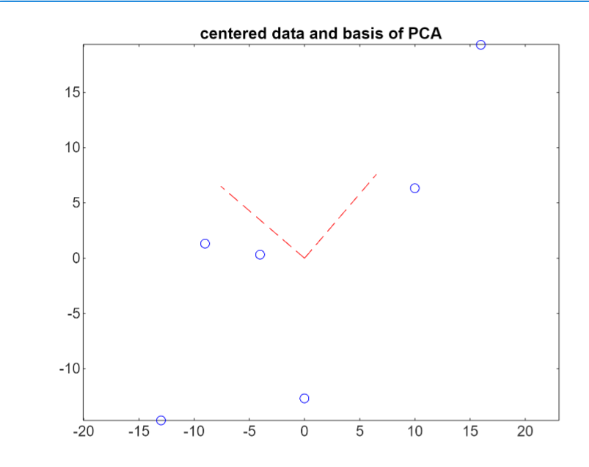
The first step is to center data, this involve computing the mean for each feature (height and weight). Then for each individual heigh and weight, we subtract the respective mean.

This results in a new matrix where each value represents the deviation from the mean, called anomaly matrix. This shifts the data sucht that the centorid becomes the origin of the reference system.

In Matlab this is done using: X = A-ones(size(A,1),1)*mean(A); % subtract the avearage of each column

Covariance Matrix §

Next, we compute the covariance matrix using the formula:

Covariance measures how two features (e.g height and weight) vary together:

• If both features are above or below their respective means simultaneously, the covariance is positive
• If one feature is above its mean while the other is below, the covariance is negative.

A large covariance implies that the two features are strongly related. For example taller individuals tend to weigh more, and shorter individuals tend to weigh less.

Computing Eigenvalues and eigenvectors of the covariance matrix §

Starting from the covariance matrix , the PCA compute the eigenvalues and eigenvectors of .

Then they are sorted in descending order.

The largest eigenvalue correspond to the principal component, which captures the maximum variance in the data. The second largest is the second principal component, and so on.

Matlab code §

A = [149 44;172 65; 153 60; 162 46; 178 78; 158 59]
X = A-ones(size(A,1),1)*mean(A); %Anomaly Matrix
C=X'*X %Covariance matrix
[PC, lambda]=eig(C) %compute eigenvalues/vectors
[variance,J] = sort(diag(Lambda),'descend'); %Sort in descending order
variance_explained = variance/(sum(variance)); %normalization of the variance

The columns of the matrix PC are the first and second principal components. The versors of the two basis are visualized in red: Multiplying the anomaly matrix by allows us to project the data into the new basis:

XPC = X*PC;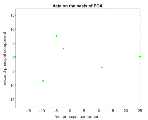

Notice how the amplitude goes from -16 to +25, that is much larger than the amplitude of the original data.

PCA and Spectral Decomposition §

Recall the what is the spectral decomposition: Spectral decomposition - eigendecomposition

Even for the PCA, we can give an interpretation as a decomposition of the covariance matrix as sum of rank 1 matrices.

Since is square and symmetric, it has real eigenvalues and eigenvectors and its spectral decomposition is:

Recall that in the spectral decomposition for symmetric matrices, the matrix composed of the eigenvector, , is an orthogonal matrix.

It follows that:

• is the -th column of i.e the -th principal component

Applying PCA to the data matrix is equivalent to applying SVD factorization to the centered data matrix . In particular we have that from and applying the SVD: it follows that

SVD and PCA Application: Eigenfaces §

Eigenfaces is a classical example of applying both SVD and PCA.

Eigenfaces represent the principal components of a database of facial images

We begin with a dataset containing 400 facial images, each with a resolution of 112×92 pixels. These 400 images belong to 40 individuals, with 10 images per person, taken from different orientations.

To simplify processing, each image is treated as a vector of pixels. Since each image has 112×92=10304 pixels, each image becomes a vector of length 10304.

The resulting data matrix has:

• Rows: 10304 (representing pixels/features)
• Columns: 400 (representing images/experiments)

The matrix is of size 10304×400.

Visualizing a face §

To visualize an image, we reshape the pixel vector back into its original matrix form. In Matlab:

imshow(reshape(W(:,36),m,n))     % reshape is necessary since an image is a column of W

This command displays the 36th image in the dataset. Using reshape we start from a vector of 10304 pixel and we obtain a matrix .

To plot the first 30 images, you need to apply the reshape for each column.

Data Representation §

Each image is a point in a space with dimensions equal to the number of pixels (10304 in this case).

When reshaping for visualization, we transform the data back into its original matrix form, but computationally, the true information resides in the vectorized representation.

A megapixel image would exist in a space with millions of dimensions

Problem Formalization §

The experiments are the images (column of the matrix), while the features are the pixels (rows of the matrix).

In this setup, contrary to previous examples, we are primarily interested in the column space .

There is no problem and the result is equivalent to considering experiments on the rows. From SVD theory, the right singular vectors of the matrix transpose correspond to the left singular vectors of the original matrix, and vice versa.

Training and Testing with 38 individuals §

Out of the 40 individuals:

• 38 individuals (380 images) are used as the training set.
• 2 individuals (20 images) are reserved as the test set

Consideriamo 38 di persone su 40. Le ultime due persone, quindi 20 foto, saranno il “test set”.

I apply a similar procedure to the one explained before in Application of the SVD on PCA.

• Compute the mean face (mean of the pxiels) avgface=mean(WA,2);
• Center the data by subtracting the mean: X=WA-avgface*ones(1,size(WA,2))
• Compute the SVD economy mode

The principal component in this example are called the eigenfaces, and they are the columns of the matrix

We use the rank-reduced SVD to represent an image that is not in the training set. Plotting on matlab we notice that with the reconstructed image begins to resemble a face, even if it does not belong to the training dataset.

Finding the Closest Image §

1. Use the entire dataset of 400 images
2. Randomly select one image
3. Find the closest image (one of the other 9 images representing the same persone).

For doing this, we us a truncated basis with components. Then we compute the cosine similarity.

This approach demonstrates that even with a small number of basis vectors, the system can accurately identify a similar image from the dataset.

---