SC - Lezione 10
Checklist
Domande, Keyword e Vocabulary
- Orthonormal basis for the row space of A
- What is the gain of this approach?
- Fundamental relationship of linear algebra (rank-nullity theorem)
- Orthogonal projector
- Is an orthogonal projector always a symmetric matrix?
- What happens if you apply twice the projection?
- Visualization of SVD
- Orthogonal directions with respect to fixed data
- Slope of a vector
- Decomposition as sum of rank-1 matrices
- k-truncated SVD approximation
- Application of k-truncated to SVD to image compression and
Appunti SC - Lezione 10
Orthonormal basis for the row space of A
It’s similar to the Orthonormal basis for the column space of A, but now we consider the row space of
Notice that in this case we have left product, in the previous case we had a right product.
The reduced dimensionality is the gain in this approach.
Orthonormal basis for the orthogonal complement of the column space of A
The last
Summary of the previous two paragraph
- The first
columns of forms a basis for the column space of , that is the range of - the first
columns of forms a basis for the row space of that is the range of
(Null space definition) How do i write the set of values X which are orthogonal to the complement of A?
The vector X is orthogonal to the columns of A
I can write:
You can also write also transposing everything like:
The null space also contains the “banal solution” where
; that is basically the origin. The orthogonal component is the vector that start from the origin. You can translate where you want it. From a mathemtically pov a vector always starts from origin
The null space of the transpose NAT in matlab and Unmr = U(:,r+1:m) are the same orthogonal matrix, in fact multiplying them you get the identity matrix.
Fundamental relationship of linear algebra (rank-nullity theorem)
Relates the number of columns of a matrix to its rank and the dimension of its null space
is the number of columns of ) is the rank of the matrix which also concides with the dimension of the column space of means the dimension of the null space of A. It represents the number of independent solutions to the equation
Orthogonal projectors of the SVD decomposition
Recall what is an orthogonal projector Orthogonal projector.
The matrix
is an orthogonal projector on the column space of (range of ) is an orthogonal projector on the row space of (range of
What can you do with an orthogonal projector?
You can project any vector onto a subspace
using the Orthogonal projector (generic) of any matrix.
What is the relationship between orthogonal projector and range of A
The Orthogonal projector is a tool to find the closest point in the range of
to a given vector. Because it project the vector onto a subspace spanned by the columns of , and the remainder lies in the orthogonal complement of
Is an orthogonal projector always a symmetric matrix?
What does it means that a matrix is symmetric? A symmetric matrix and you compute its transport you get the same matrix.
Or, an equivalent definition is that the
This property, that an orthogonal projector is always a symmetric matrix, can be easily demonstrated. Consider the matrix
I interchange the two terms because when i do the transpose operation on a product, i need to interchange the two, so it becomes:
Idempotent property of orthogonal projectors
What happens if you apply twice the projection? Like the square of the matrix. So a projector is symmetric but when you compute the square so you apply it twice you must have the projector itself. Since a double projection is equivalent to a single projection.
This can be demonstrated easiliy:
Let
Notice that
(This property is called idempotent)
Visualization of SVD
We use our function VisualizeSVD_LE
This function generates a random 3 by 2 matrix. You can multiply this by a vector of two component and you get a vector into three dimensional space. It’s a transformation from 2 to 3 dimension.
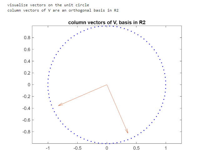
the three dimension vector stays in the two dimension subspace generated by the two columns of the matrix.
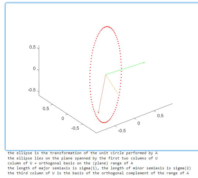
In the image the circle is transformed in an elipse. The two orange vectors are the first two element of the column of U and the green is the third column of
Identifying orthogonal directions with respect to fixed data
Consider 10 points on the line 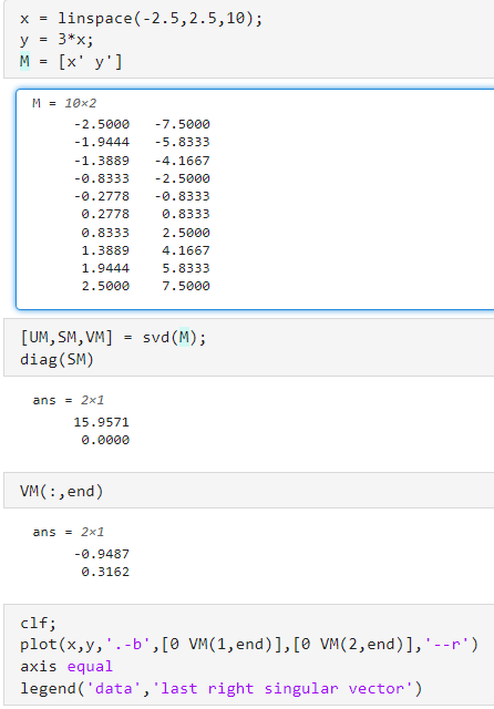
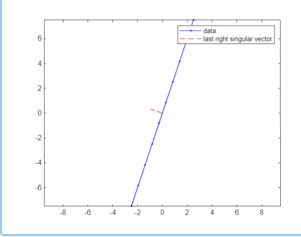
We now observe that the basis of the orthogonal complement of the row space is useful for identifying orthogonal directions with respect to fixed data.
Slope of a vector
The slope of a vector is the rate at which the vector rises (changes in the vertical direction). In the case of a 2D vector, like in our example
The slope is:
The slope of VM(:,end) is computed as VM(2,end)/VM(1,end) because it’s a
Decomposition as sum of rank-1 matrices
Let
One of the most important result is the k-truncated SVD approximation
k-truncated SVD approximation
The idea is to instead of summing them, i just stop at an index
There is a very important theorem in data analysis, that says that
You have an expression that is computed with the 2-norm of set of singular values.
Exercise
- Take a picture of yourself
- Send it to laptop (must be JPEG format)
- Give it a name and add it to the path
(Vedi SC_ONLINE_Tutorial_06_Applications_SVD.mlx)
Il codice è questo cmq, lo ha fatto vedere solo a lezione
img = imread(...) %qua devi mettere il nome del file
img = rotate(img,-90)
img_gray = double(img_gray)

[U,S,V]=svd(img_gray)
k=50 %(k=50 truncated SVD)

img_reconstructed = U(:,1:k)*S(1:k,1:k)*(V(:,1:k)';

%now to display it as picture:
figure;
sublot(1,2,1);
imshow(uint8(img_gray));
title('original image');

subplot(1,2,2);
imshow(uint8(img_reconstructed));
title('approximated image with k=50');