SC - Lezione 14 - Systems of non linear equations, Jacobian Matrix, Newton methods for NLS, Fixed Point Problem

---

SC - Lezione 14 §

---

Checklist §

Checklist

Domande, Keyword e Vocabulary §

• vector function
• vector-valued function
• Contour Plot
• Newton Method for non-linear systems
• Jacobian Matrix
• What’s the difference between gradient and Jacobian?
• Taylor Series
• Quadratic Convergence of Newton Method
• Newton-like Method (o damped Newton method)
• Damp parameter
• Search Direction
• Fixed Point Problem for vectorial-valued functions
• Contraction Mapping
• Dominant eigenvalue of the Jacobian matrix of
• Relationship between and Fixed Point Problem

Appunti SC - Lezione 14 - Systems of non linear equations §

Let be a vector function with components with x in

Let us consider this equations:

We have that n=2 and the variables are and You have n=2 equations and x and y are the unknowns.

fsolve §

In matlab we can use this command to solve the non-linear system

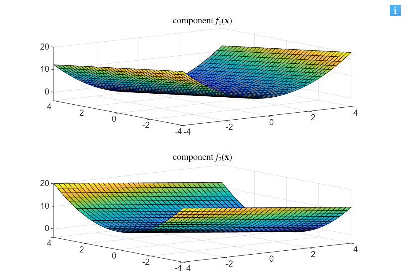
contour plot §

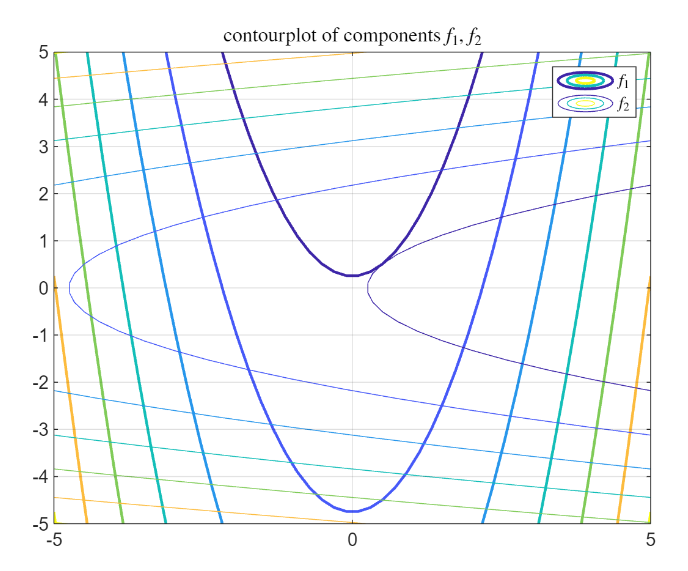Consider the first function that represents a surface. The contour plot is generated by taking a set of planes parallel to the domain and intersecting them with the surface. Each intersection creates a contour line, which is then displayed in the plot

So the graphical solution of 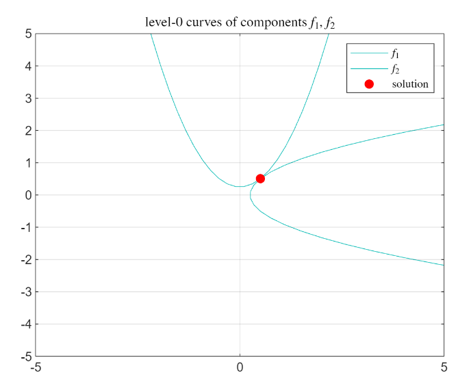it must stays on the level zero of both components and . So if we look at the counterplot of components again, what are shown are the level zero. So the geometrical interpretation of the solution is the intersection of two zero lines of both and .

Newton Methods for solving non linear system §

A non-linear system can be solved by Newton’s method for non-linear system, which is a straightforward generalization to a multidimensional context of the Newton’s method for univariate functions.

We recall that for 1 variable we have that:

What we consider now is just this but generalized to multivariable context.

Jacobian Matrix §

Since we are in a multivariable context, we must consider the Jacobian Matrix of at

Jacobian Matrix

It’s the matrix with all the first-order partial derivatives of a vector-valued function.

For a function the jacobian matrix is an matrix given by:

J = \begin{bmatrix} \frac{\partial f_1}{\partial x_1} & \frac{\partial f_1}{\partial x_2} & \dots & \frac{\partial f_1}{\partial x_n} \ \frac{\partial f_2}{\partial x_1} & \frac{\partial f_2}{\partial x_2} & \dots & \frac{\partial f_2}{\partial x_n} \ \vdots & \vdots & \ddots & \vdots \ \frac{\partial f_m}{\partial x_1} & \frac{\partial f_m}{\partial x_2} & \dots & \frac{\partial f_m}{\partial x_n} \end{bmatrix}$$

---

What's the difference between gradient and Jacobian?

The Gradient is a vector of partial derivatives of a scalar-valued function The Jacobian is a matrix of the partial derivatives a vector-valued function

The gradient is a special case of the Jacobian when the function has a single output

For example, consider a simple function with two variables; it has two partial derivatives, which can be combined to form the gradient vector.

When dealing with a vector-valued function, each element of the vector has its own gradient. This idea extends to the Jacobian matrix, which is composed of the gradients of each component in the vector-valued function.

The Jacobian matrix is very important in Artificial Intelligence

So the formula for solving these non linear system is:

The rows of the Jacobian matrix are the gradient of the components of .

Deriving the method from Taylor Series §

The method can be easily derived from the Taylor series of a vectorial function F at :

omitting the second order term and looking for the next approximation as a solution of we have that:

The second order term represents the error of the approximation and is omitted because we don’t know it.

The method can be written, at each step , in a more efficient way as solution of the linear system:

Such that the update solution will be:

Note that:

Some properties §

the newton’s method is a local method with quadratic convergence rate. It converges and the number of correct digits of the approximations doubles at each step.

The Newton’s method for nonlinear systems requires a function for computing the Jacobian matrix of the vector function as input argument.

JF = @(x) [2*x(1)  -1; -1  2*x(2)];
maxiter = 30; xiniz = [0.1,0.2]'; tol = 1e-8;
rNEW = NewtonSystems(F,JF,xiniz,tol,maxiter)

Then we have another example in three dimensions

Damped Netwon’s Methods (Newton-like method) §

A useful variant of Newton’s method is the damped Newton’s methods, that consists in considering in the updating formula a parameter that has to be computed at each step in order to avoid that the new approximation is too far from the previous one.

is called the learning rate in Machine Learning (backlink)

must not be too big otherwise the method doesn’t converge.

Method Definition You compute first the correction as in Newton Method:

But instead of using it all you just use a part of it:

It’s called the damp parameter in this case.

is computed at each step as the minimum of one-variable function:

How to compute this parameter? It’s very easily theoretically because what you want is just that your functions becomes zero. At a certain point you compute the norm for example 10, then you compute the correction that solves this system.

In the following approximation the norm of the function must be less than 10 and so on with each iteration.

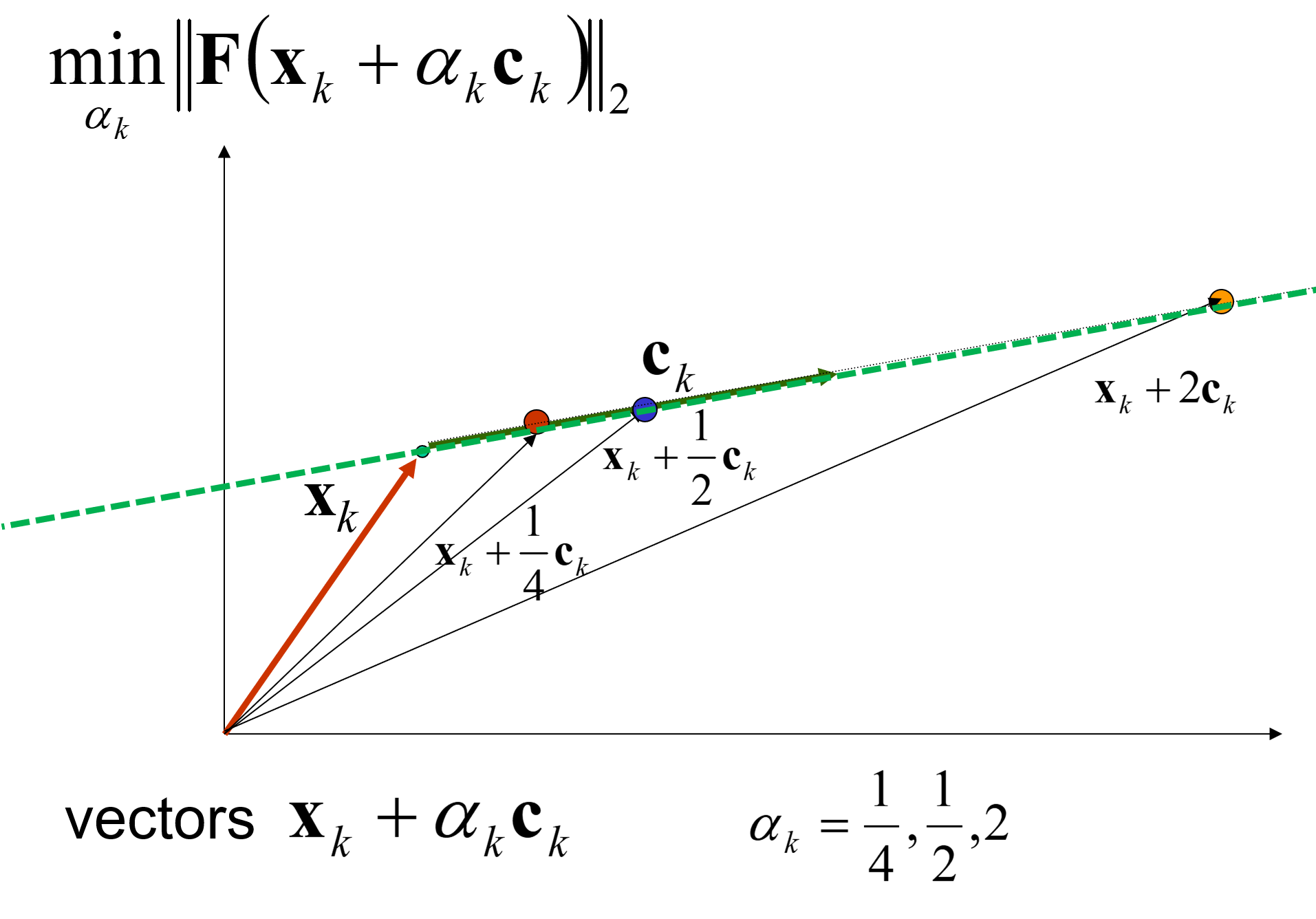
What is the best way to do that? minimize this quantity:

Remember this is a function of one variable, a scalar function, so you want to minimize respect to the choice of this scalar function that is very easily to do.

is the search direction, that is the line on which the next approximation is searched.

Fixed Point Problem §

Let be the fixed point problem defined as

nota: è una funzione vettoriale

Fixed Point of a function

link

The fixed point problem can be solved by the fixed point method:

which is a local method with linear convergence rate.

Suppose that you have a solution in a certain set: . If you start from any point in this set you have the method converges to solution if the function has this particular property

Contraction Mapping In :

Means that is a contraction mapping in .

if is differentiable near the solution, then a sufficient condition for the convergence of the fixed point method is that the modulus of the dominant eigenvalue of the Jacobian matrix of is less than 1.

The modulus of the dominant eigenvalue of is called spectral radius

TL:DR if the spectral radius of is such that then it’s a sufficient condition for the convergence of the fixed point.

F(x)=0 and Fixed Point Problem §

The problem can be transformed into an equivalent fixed-point problem:

Is equivalent to

We see in matlab that the method diverges since the spectral radius of is greater than 1, and this implies that we should expect that the method doesn’t converge.

Matlab code:

G = @(x) [x(2)^2+0.25; x(1)^2+0.25];
xiniz = [0.6,0.6]';
x = xiniz;
for i = 1:100
    x = G(x);
end
x
JG = @(x) [ 0  2*x(2); 2*x(1)  0];     % Jacobian matrix of G at point x
[X,L] = eig(JG(r))

---