---

SC - Lezione 16 - Gradient Descent Methods, with momentum, ADAM, Stochastic, Levenberg-Marquad §

---

Checklist §

Checklist

Domande, Keyword e Vocabulary §

• Gradient Descent Methods
• Standard Gradient Descent
• stepsize parameter - learning rate
• searching direction
• minimization
• convex functions
• Hessian Matrix
• Property of the hessian matrix
• Rate of convergence
• Implication of the rate of convergence for Gradient Descent Convergence Speed
• Minimization path of the gradient descent with optimal choice and constant learning rate
• convergence
• zig zag pattern
• Gradient Descent with momentum
  • weighted average between the gradient and previous value of
  • Momentum
  • Momentum Coefficient
• ADAM method
• Stochastic Gradient Descent
  • Computing Gradient is expensive
  • Samples / Batch of Samples
  • Gradient Approximation
  • Epoch
  • With Replacement vs without replacement
• Newton Method
• Levenberg-Marquadt Method

Appunti SC - Lezione 16 §

Gradient Descent Methods §

Standard Gradient Descent §

It’s an iterative process.

• is the stepsize parameter (in AI called the learning rate); it can stay constant or be selected at each step (and we have several techniques for that such as backtracking or optimal choice)
• is the searching direction at step k.

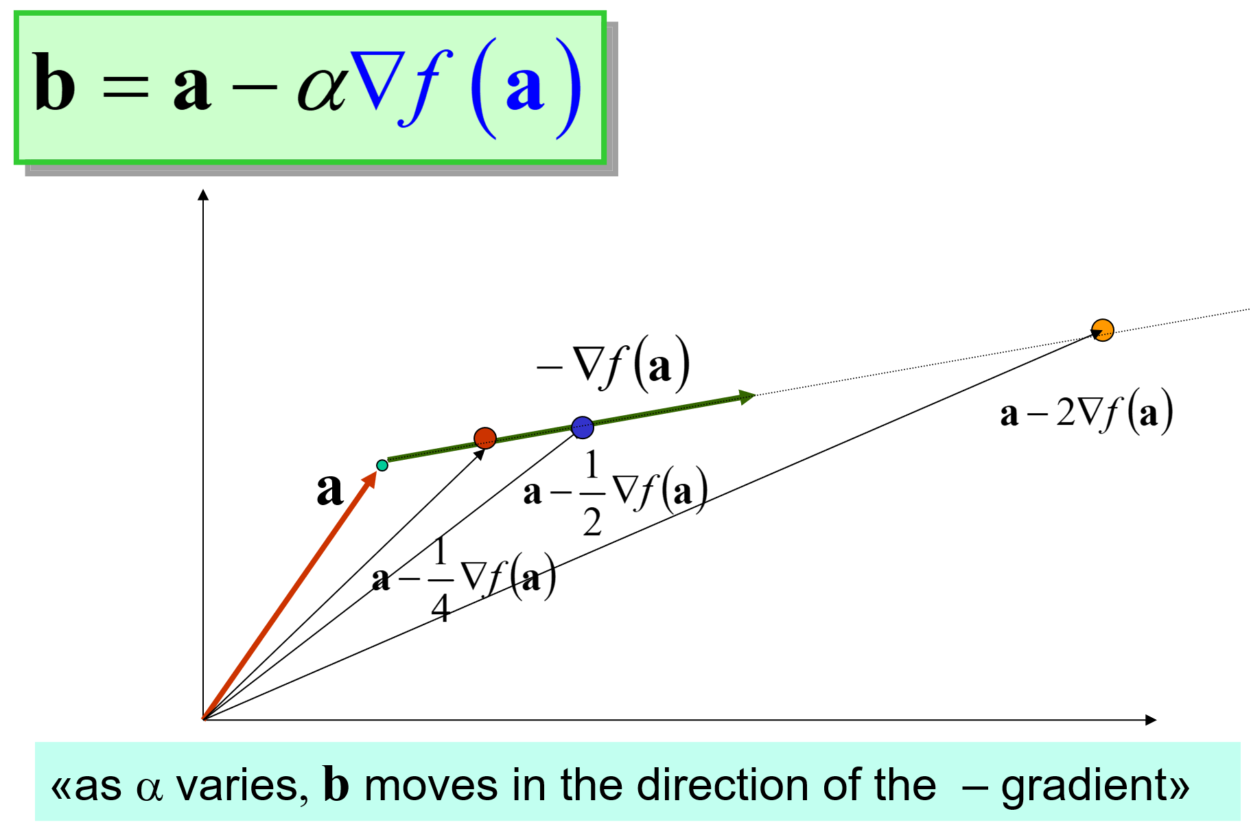
Selecting : Optimal Choice §

At each step we want to solve a subproblem of minimization.

We want to find the that minimizes evaluated at ””

Convexity §

Convex function: concavity is up

Convexity is of great help in minimization: if we have to determine the minimum of a convex function defined on a convex set then we know that two isolated solutions cannot exist.

If the function is convex: x and y are minimum points of f then all points z between x and y are also minimum points. If the function is strictly convex in , then there is a unique minimum point. Also, its Hessian Matrix is symmetric and positive

What is an Hessian Matrix?

A square matrix whose entries are the second partial derivatives of

Property of the Hessian Matrix: the eigenvalues of the Hessian matrix determine the actual speed of convergence of the GD method. This is expressed by the ratio:

where s are respectively the min and max eigenvalue

Rate of Convergence:

Explanation

• is the function value at -th iteration, and it’s the function evaluated at the next iteration
• is the minimum value of or the function evaluated at the optimal point r
• and are constant that we saw in the above ratio
• is a value between 1 and 0

Implication of the Rate of Convergence for Gradient Descent Convergence Speed The Hessian describes the curvature of the function. (Recall: it’s the matrix of the second derivatives, in a single parameter function the curvature is described by the second derivative).

If (i.e, ) then the function has very different curvatures in different directions (eigenvectors), which can lead to slow convergence of the GD method. This imply that the GD algorithm may take very smalls steps in directions where the curvature is high and larger steps in directions with low curvature. Conversely, if the eigenvalues are similar, the function is more well-behaved, and GD can converge more quickly.

Practical example of GD §

Now we apply the GD method to the objective function whose gradient is and the solution is

We see two interpretations in our matlab example: one with optimal learning rate and one with constant one 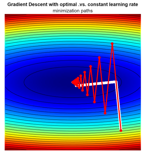In white there is the minimizaiton path of the gradient descent with optimal choice, while in red there is the other one. (The Steepest Descent Method that implement standard GD)

The lesson here is that the one with optimal learning rate converge faster to the final solution . The one with the constant learning rate shows a zig zag pattern and is slower.

In real application we can’t use the gradient descent with optimal choice because it costs too much.

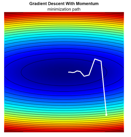
Gradient Descent with momentum (GDM) §

How can we avoid the zig zag behavior? One solution could be the Gradient Descent with Behavior that is defined as:

What is ? It’s called momentum and it’s obtainted by the formula:

• it’s a normalization factor, that multiplied by computes the weighted average
• (between 0 and 1) is called momentum coefficient, and control how much of the previous gradient’s direction influences the current update

It’s a weighted average between the gradient and the previous value of . It’s a sort of history of the pattern along the path.

More formaly we can say that, by considering past gradients in the searching direction can naturally adapt to the behavior of the objective function, tuning the updates according to the geometry of the surface.

These minimization methods are usually used in the learning rate of ML algorithims.

The advantages of the GDM are: faster convergence because of the reduced oscillations and a better handling of curved surfaces, making it less prone to being trapped in local minima.

ADAM method - Adaptive Moment Estimation §

It’s another variant of the Gradient Descent for smoothing out the minimization path.

Definition:

We have two different “variables” now: and is the same as defined before: and as said before represent a sort of history of the pattern.

Instead, is defined as:

And it’s a sort of history of the square 2-norm of the gradient.

Notice that we are multiplying the gradient transpose of by the gradient of . The result (a vector) is weighted by and it’s summed by which represent the previous parameter.

When put in the ADAM method definition, the value is squared, so it’s effectively a squared norm

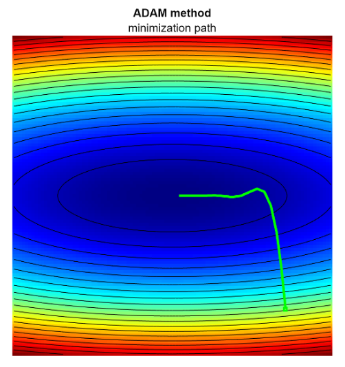
the ADAM indirectly adapats the effective learning rate by means of moving average of squared 2-norm of gradients. In fact, it is largely used in large scale AI Applications and its variants.

Stochastic Gradient Descent §

It’s a very important method widely used in the field of Machine Learning and AI, for training Neural Networks.

Why it is used: when dealing with very large datasets, computing the gradient of the objective function over the entire dataset is computionally expensive. So we cannot used traditional GD methods.

Idea: The Stochastic Gradient Descent works by updating the variables of the objective function using a single sample (or a batch of samples) at time.

This approach introduce noise, as each sample only provide an approximation of the true gradient. But despite this, the SGD often leads to faster convergence over large datasets.

Suppose that we are training a Neural Network and we have the following objective function (that we called Loss Function in Machine Learning 1):

• is the vector of the parameters of the NN
• is the size of the training set
• is the individual loss associated to the -th sample of the training set. But i don’t want to use all of these samples: i want to use a much smaller dataset of this learning set.

Note: the loss function of a NN is a measure of how well the network’s predictions match the label outputs over the training set

The pure stochastice gradient descent just pick one element, randomly picked. And this will be used instead of .

In general, considering a subset of elements randomly choiced we can write:

So are random numbers in

The SGD with this minibatch is defined as:

• ”” Means that you compute the gradient of just a part of the sum.

Epoch A complete pass of the entire training set (backlink a lezione di machine learning). If each iterations uses a mini-batch of samples, then one epoch consists of iterations

What can we do in pure SGD is to implement a for loop over the entire dataset and pick just a random sample and then at the end of the for loop you have finished an epoch and you can use another epoch.

The number of epochs of course have a great influence on the total cost of the process, usually the number of epoch is in the order of 1000s.

SGD with Replacement and without Replacement §

SGD can be implemented with replacement or without replacement.

• without replecement: select each sample from the training only once per epoch
• with replacement: the same sample could be choosen more than once for epoch

For a NN without Replacement is better, why?

The one without replacement is generally preferred because: it makes more efficient use of data, it improves the convergence stability and reduce the variance in gradient estimate

Example 1 §

Suppose that we have a function that is a sum of two functions:

We want to minimize this function.

At each step, I randomly select one of the two functions to compute the gradient. For the experiment, we repeat this process 50 times: running 1000 iterations of SGD, where at each step, one of the two functions is randomly chosen, the gradient is computed, and the solution is updated accordingly.

Then by plotting all of these stuff: 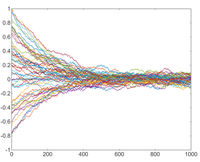We notice that Each line is a sort of minimization path and we notice that they all converges to 0.

Starting from any point, this method quickly brings you close to the solution, but it doesn’t fully converge. This is an useful property for avoiding overfitting.

Another key thing is that we can stop before reaching 1000 iterations, as this brings us near enough to the solution without getting too close, which would otherwise lead to overfitting in neural networks.

Example 2 §

Da fare

Consider a simple mimicking scenarion of the learning process of a Neural Network. The objective function (cost function) depends on two parameters: and and is made up of three quadratic terms:

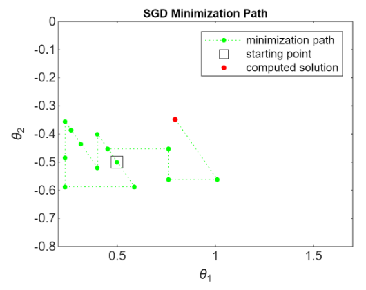
Notice that it’s not true that the next approximation is less than the value at the previous approximation because we are considering only a part of it, but the general behavior is that it descends.

This behavior also depends from the choice of

In real bheavior applications our function is not necessary a convex, so we could have local minimum. We want to avoid this and we want to go in a stochastically way to the global minimum. And we want to do this by choosing random small batches. This avoid that we can get stuck is local minimum.

Newton and Levenberg-Marquadt Methods §

It’s another method for solving minimization problem. This method can be derived from the Taylor series expansion of a scalar multivariate function :

By omitting the term and setting:

gives the Newton method for minimization.

Let’s consider the objective function and we want to use the Newton’s method for minimization, so:

Recalling the Newton’s minimization method §

The newton minimization method for a function of one variable it can be seen in different ways like the standard newton methods such that:

when you want to move to the multi dimensional case we expect that we need to use an entity that correponds to the same in multidimensional and it is the gradient (that is the vector of partial derivatives). We use the Hessian matrix, that ofcourse cannot go at the denominator, so it will be appear as the inverse of the hessian. And how can we derive this method?

Recall first the (1D) classic method:

but we cannot consider this approach and we use the Taylor Series at :

Now, if is fixed, so it cannot change. The only thing that can change is so i have to minimize this variable so the problem becomes:

And what i get will be the correction to apply to in order to get What’s the minimum of this? I have to compute the derivative respect to and put i to 0 So doing the derivative we get:

Now generalizing this formula to several variables we have:

Note that is a scalar function but is a vector of variables. is a number, is a scalar number, is a column vector by a matrix and it’s a scalar. From a dimensionality point of view we have checked that the right side of the equaiton is a number as we expect by at the left side

I want to minimize like before. First i don’t consider the last term so i write:

is a quadratic function of the variable that is the element i want to minimize. To minimize this from a theoretical pov i have to look at the value of that makes the gradient of equal to zero:

By putting the term on the right side, and multiply both sides by the inverse of the hessian matrix then i get the c:

This is a system of linear equations

It’s the general formula that we consider. It just uses the gradient and the hessian matrix. I start from an initial approximation, solve this system of linear equation and compute the following step as:

And this is much more faster than gradient descent method. But it’s very difficult to apply in situations where there is a vector of billions of components because we have an hessian matrix with billions of rows and columns.

Levenberg-Manquardt Method §

• Gradient Descent Methods
• Newton Methods

It’s a combination of the Gradient Descent method and Newton’s minimization method. We want the average of both the methods:

The idea is that, while gradient descent relies solely on gradient information, Newton’s method incorporates the Hessian, thus utilizing information about the function’s curvature as well. This means that, instead of using just the gradient as in gradient descent, Newton’s method considers both the slope and the curvature.

So instead of using just the gradient in the GD:

I want to combine it with the newton:

We put both together:

This is the basic version of the Levenberg-Marquardt (L-M) Method. It inherits some of the limitations of the two methods it combines: it is prone to overfitting (as we saw, the stochastic approach helps mitigate this), and it becomes impractical for high-dimensional problems due to large data requirements and the computational burden of handling large Hessian matrices.

L-M can be seen as an improvement of the Gradient Descent algorithm, since the information on local curvature (Hessian) of the objective function is also considered, in addition to its gradient. Note that L-M is a local method with less than quadratic rate of convergence. However, it may converge faster than traditional GD method in regions where Newton’s method might diverge.

Exercise

Implement the gradient approximation variant

---