SC - Lezione 21 + 22 - Automatic Differentiation, Discrete Fourier Transform introduction
Domande, Keyword e Vocabulary
- Symbolic Differentiation
- Automatic DIfferentation
- Computational Graph
- Reverse Mode
- First and second phase of the reverse mode
- Adjoint Variable
- Backpropagation and Neural Networks
- Loss Function
- Backward Pass
- Gradient Descent Step
- How many update we do of the parameters, at each epoch, if we use the Stochastic Gradient Descent?
- ReLu Activation Function
- Recap Complex Numbers
- Imaginary Unit
- Modulus
- Complex Conjugate
- Polar Representation
- Euler Formula
- Special Case
Appunti SC - Lezione 21 + 22 - Automatic Differentiation, Discrete Fourier Transform introduction
There are 3 approaches to compute derivatives:
- Numerical differentiaton as we saw in SC - Lezione 20 - Computing Derivatives Finite Differences
- Symbolic Differentiation
- Automatic Differentiation
Symbolic Differentiation
Symbolic differentiation manipulates mathematical expressions to get the exact symbolic expression of the derivative.
Basically you take the expression, you break it into smaller parts, differentiate according to the applicable rules, then recombine the differentiated parts according to the rules of differentiation.
Symbolic differentiation is very complex.
Automatic Differentiation
The first key difference of AD with ND is that it computes the derivative of a function at a specific point.
AD methods takes as input a differentiation point and the symbolic expression of the function or a program that evaluates the function at any point. The output is the exact numerical value of the derivative at the provided differentiation point.
How does the AD works? It applies repeadetly the chain rule from Calculus to basic functions that compose the input function (or the lines of the program that implements such function.
An example of program that we saw in the Matlab file is:
function [f, grad] = simplefg(x)
        f = (x(2) - x(1).^2).^2 + (1 - x(1)).^2;
        grad = dlgradient(f,x);
end
We used then dlfeval matlab function to eval this ^.
The problem of the AD is that it provides only the value of derivative in a point, if you want the value of the derivative in more than one point you have to run multiple time the procedure.
Forward and Reverse mode in Automatic Differentiation
Forward mode evaluates a derivative of a function at a given point by performing elementary derivative operations concurrently with the operations of evaluating the function itself. AD software performs these computations relying on a computational graph that represents the function to be differentiated
Reverse mode (backtracking) works by reverse traversing the graph.
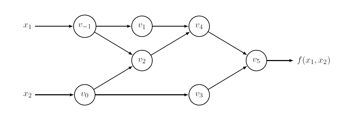
Computational Graphs
A computational graph represents the sequence of elementary operations and basic functions that are executed to compute the output of a given function from its inputs. The components of a computational graph are:
- nodes: represents a basic operation like addition, multiplication, sin, sqrt
- edges: dependencies between operations or the flow of data between nodes
- leaves: are nodes without incoming edges
- root: final output node of graph
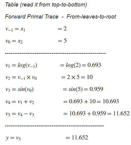
Example
Consider the evaluation point
is:
Reverse mode
It propagates the derivatives from the leaves to the root of the computational graph.
The Reverse mode requires to complement each variable
adjoint variable: equivalent of the update of (neural) network in learning phase
In practice, in reverso mode we have a first phase where we build the computational graph, and intermediate variables
Example
Consider the previous computational graph:
We see that
as
And this is in the first phase. We saw that in the second phase we replace derivatives using the adjoints variables:
Generalization of the adjoint variable
where the summation is extended to all the intermediate variables that have an incoming edge from variable
Backpropagation and Neural Networks
We consider a Neural Network with 1 layer We want to describe his learning by computing the parameters of the NN using a training set
We show in details, using mathematical notation, how to compute an update step of Gradient Descent using the partial derivatives (adjoint variables) computed by the backward pass.
Components of the Neural Networks
- The linear layer:
- The weight matrix
is the unknown, the paramter to compute is the bias vector and is also unknown is the input vector
We consider the following loss function:
The given loss function is a mean squared error (MSE) loss, which measures how well the neural network’s predictions match the true target values.
Note that:
The loss function is:
- The term
represents the error between the predicted value and the true target for a single sample . - Squaring the error ensure that it is always positive and penalizes larger errors more than smaller ones
- Taking the mean of the error
ensures the loss reflects the model’s overall performance across the dataset, not just on individual samples.
Scalar functions vs Vector function
Note that, if
Now we consider the backward pass and the gradient descent step
Backward pass
During the backward pass we compute the gradient of the loss function
Before we saw automatic differentiation, if we want to apply it in this case, we need to consider the Neural Networks as a computational graph.
- gradient respect to
: - gradient respect to b:
Gradient Descent Step
- Recall Gradient Descent
Given the learning rate
The update of b:
with each update we want to reduce
Epochs and comparison of GD with Stochastic GD
After these two steps, I have completed one epoch. Now, we start another epoch, using the same training set but with updated parameter values. We repeat each step and continue this process for as many epochs as needed.
How many update we do?
In the case of the traditional Gradient Descent, we perform one update per epoch, as the parameters are updated only after processing the entire training set.
What if we consider the Stochastic Gradient Descent, with a minibatch of size 1? We do
The Stochastic Gradient Descent is more accurate because you make more update and adjust the parameters after each sample.
ReLU Activation Function
In the end, we just want to sketch what happens when we introduce a simple but important change to our NN, adding a ReLU activation function to each neuron in order to obtain a non linear network:
ReLU has to be considered when computing the gradients:
now must include the ReLU derivative: now must include the ReLU derivative so that:
Where
The derivative of the ReLU function is:
Modern deep learning frameworks, such as TensorFlow and PyTorch, automatically construct and manipulate computational graphs and use Automatic Differentiation for efficient computation, gradient calculation, and scalable model training on various hardware architectures.
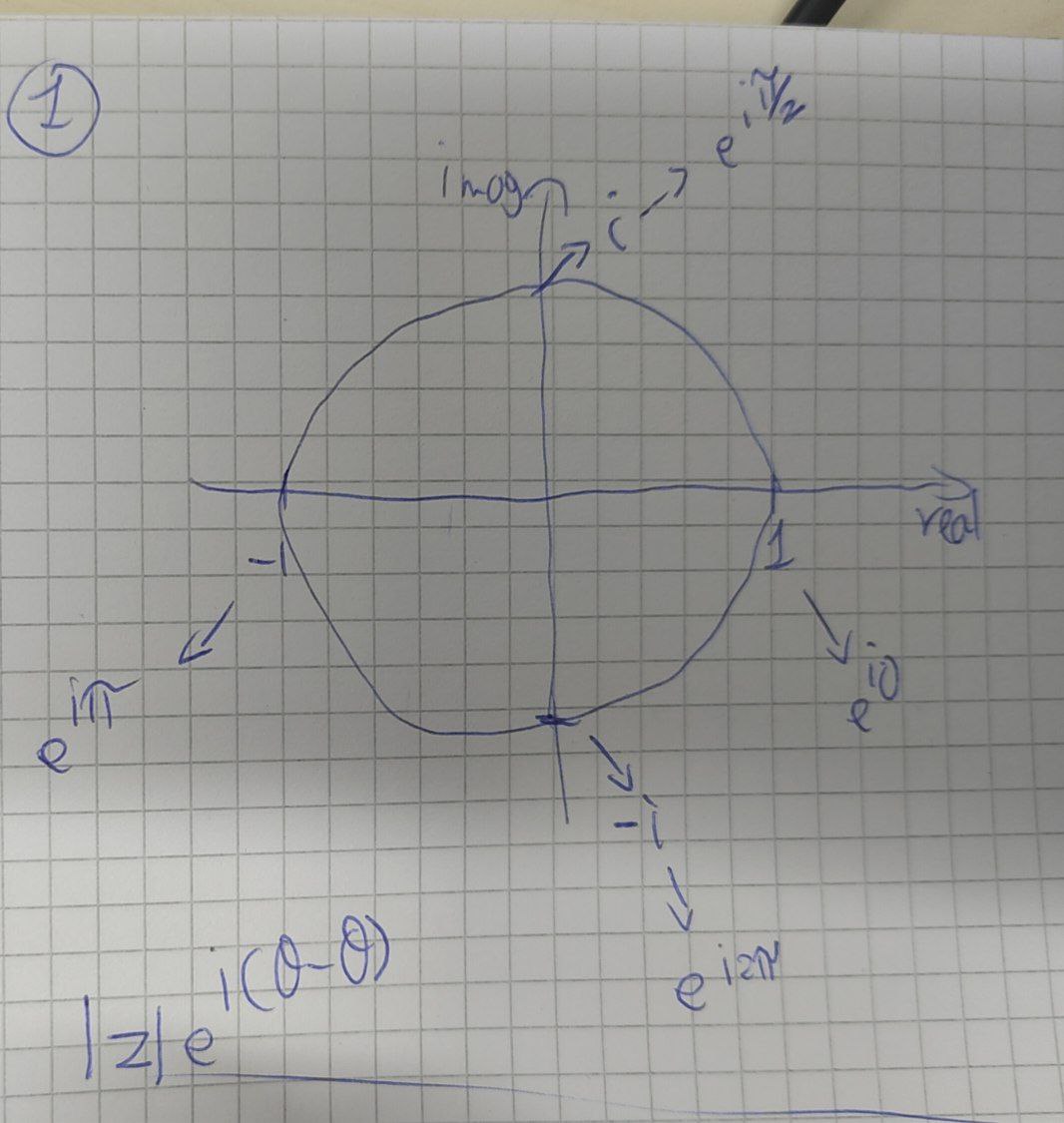
Discrete Fourier Tranform
Recap Complex Numbers
- Imaginary unit
= or - Complex number is of the form of
where is the real part and the imaginary part - The modulus of a complex number it’s his distance from the origin in the complex plane:
- Complex Conjugate:
- The phase of a complex number is the angle
that the vector representing the complex number makes with the real axis - Polar representation:
Euler Formula: for any real number
Special Case: note that when