---

SC - Lezione 23 - Root of Unity, DFT definition, Frequencies, Amplitude Spectrum, DFT as matrix-vector product §

---

Checklist §

Checklist

Keyword §

• Root of Unity
• Discrete Fourier Transform
• Magnitude (amplitude) and phase
• DC component
• Fundamental Frequency Component of the signal
• Sampling Rate and Sampling Frequency
• Frequency Resolution
• Sampling Period
• Recap on Frequencies
• Amplitude Spectrum
• Conjugate Symmetry
• Single-sided spectrum
• Quasi-unitary property
• Hermitian matrix

Appunti SC - Lezione 23 §

Root of unity §

It’s a number called It’s defined as:

Which means that it has magnitude 1 and angle

which is the 4th quadrant (see recap complex numbers)

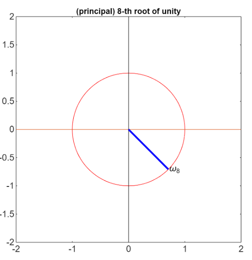
Property of the root of unity: if we raise omega to N we have that:

Omega N is the N-th root of unity. If you raise this number to N you get exactly 1

Alternative Notation

The definition is the same as if you use the minus sign. The minus sign is used in the fourier analysis. Usually another notation is without the minus, that is also good but we prefer the minus definition.

Raising to any powers from 0 to generates all the -th roots of unity

Consider the previous image: It’s , whatever 8th root of unity you pick in the circle, incresing powers of can be obtained just increasing the angle by , We may observe that:

There are just distinct root of unity (8 in the example)

Discrete Fourier Transform §

What it is used to: analyize discrete signals Idea: transform samples (such as sound waves) from a time domain to a frequency domain

Definition: The input of the DFT is a finite, discrete signal (a vector) and the output is a finite, discrete signal (a complex vector) in the frequency domain.

The input to the DFT is a vector of that represents a discrete signal The output is a vector that represents the same signal in the frequency domain.

the k-th element of is defined as above. is multiplied by the root of unit. In fact we can write in a more compact form:

for

Note also that if , then

Each element corresponds to a specific frequency component in the signal. The frequency associated with is

Recap of the elements of a signal §

Magnitude: the magnitude of each quantifies the amplitude of the frequency component within the signal, indicating its strenght and presence Phase of represents informations about the sinusoidal components at this frequency Direct Current Component: is the DC, representing the average value of the entire signal. It doesn’t change over time, so it is associated with a frequency of 0;

Fundamental Frequency Component of the signal: that is the smallest non-zero frequency which is indeed in terms of cycles per sample, when the total number of samples is considered over a unit time interval.

Note that we defined the frequency of the element with , if we consider , we obtain , that is because it is called the fundamental frequency component of the signal.

is the frequency in cycles per sample, that is the number of complete oscillations of the signal between each pair of consecutive samples.

The physical frequency depends on the sampling rate and is equal to

Example §

I have the signal represented by the function .

• is the frequency of the cosine wave; it oscillate cycles per second
• is the time in which we observe the signal, goes from 0 to 1

if , it makes 5 oscillations when goes from 0 to 1

Sampling Frequency: to digitalize this signal (infinite to finite), we decide the value that is the sampling frequency (or sampling rate) which is the number of samples taken per second from the continuous signal to convert it into a digital signal.

For example if , it means that that 1000 samples of the continuos signals are taken every second. If we sample a signal at for seconds, we will have samples

Frequency Resolution: the spacing in frequency between individual points in Time step / sampling period: is the time interval between consecutive samples in the digitalized signal and it is the inverse of the sampling rate: .

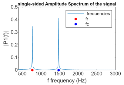
Amplitude Spectrum §

It is defined as

• is the vector of moduli of the components of the complex vector (to which we applied the DFT).
• is the number of samples used for sampling the signal.

It shows how much of each frequency is present in the signal, providing insight into the signal’s frequency content and strength at each frequency component.

We consider in an example this signal: signal = sin(2*pi*60*t) + 0.9*sin(2*pi*120*t); which is given by the sum of two sinusoids.

Conjugate Symmetry (or Nyquist Index) §

There is a symmetry between negative and positive frequencies, since mathemtically they are one the complex conjugate of the other.

So they carry the same information and it’s redundant to consider both in practical application. We consider only the single-sided spectrum

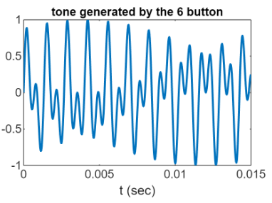
Example of analysis of audio signals §

Classical example of the Touch-tone telephone dialing, that uses the dual-tone multi-frequency signaling (DTMF) standard, associated with each row and column is a frequency.

The tone generated by pressing the button in position is obtained by superimposing the two fundamental tones with frequencies fr(k) and fc(j).

• fr is the frequencies of the rows
• fc is the frequencies of the columns Like before we make the sum of the two frequencies and .

Example 2 §

Now instead of just press 1 button i press a sequence of buttons, 11 digits. The recording is this:

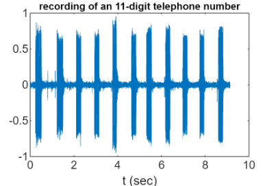
If we compute the DFT we see that: 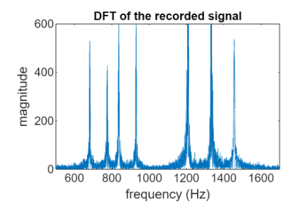There are 7 peaks, corresponding to the seven basic frequencies but we cannot determne the individual digits. We don’t know which frequency come first, we don’t know the distribution over time and this is the main problem over DFT. It make sense, because when you transform a signal from the time domain to the frequency domain, and you analyize this signal, you don’t have the information about time.

We have to break this signal into 11 equal segment and anaylize them separately.

DFT as matrix-vector product §

The DFT can be interpreted as matrix-vector product.

• is the column vector of N components of input
• DFT matrix , square
• is the output

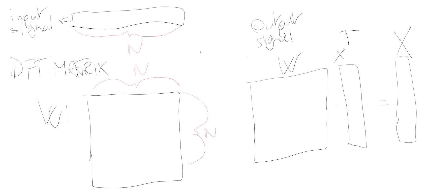
The generic entry of is defined as:

What we are doing is projecting using as transformation, you project onto a basis of the cosine function that is an orthogonal basis.

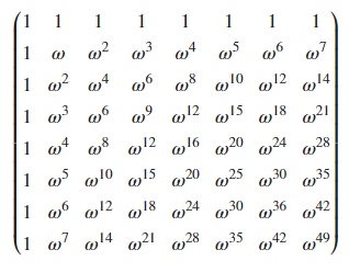
For example in Symbolic Matlab here is the DFT matrix (order 8):

Hermitian Matrix (or conjugate symmetric) §

A complex matrix is hermitian if holds:

It’s the complex correspective of the symmetry.

If is Hermitian then the elements on the main diagonal must be real numbers, as the complex conjugate of a real number is the number itselfs; The element in the position must be complex conjugate of the element in the position for all

DFT Matrix is not Hermitian since and are not equals. But it shows a conjugate symmetry property:

Conjugate Symmetry Property and Quasi-unitary property §

Conjugate Symmetry Property: recall that the overline means the conjugate of each entry of . This in fact is just the usual concept of symmetry for real matrices.

Such conjugate symmetry of leads to the conjugate symmetry in the frequency domain representation of real-valued time-domain signals.

Quasi-unitary property: The DFT matrix enjoy of the following property:

---