SC - Lezione 30 - 2D CWT, Discrete Wavelet Transform and its inverse, Fast Wavelet Transform Algorithm

---

SC - Lezione 30 §

---

Checklist §

Checklist

Domande, Keyword e Vocabulary §

• 2-D Continuos Wavelet Transform and its inverse
• Comparison with the 1D Wavelet Transform
• Two translation parameters
• Orientation Parameter
• 4D Tensor
• Algorithm for Discrete 2D Wavelet Transform
• Exercise: facial feature extraction with 2D-CWT
• small scales, larger scales, different orientations impact on facial feature extraction
• Discrete Wavelet Transform DWT
• Computational complexity of the DWT
• Definition of the DWT
• Discretization of a wavelet
• Fast Wavelet Transform Algorithm
• Approximation Coefficients Vector and Detail Coefficient Vector
• Decomposition Levels
• Downsampling
• Final Decomposition and DC component
• Application to a random simple signal
• Application to a more complex signal
• Frequency Bands and Octaves
• Octave
• Deeper Insights into the computation of single-level decomposition
• Haar mother wavelet and Haar sampling function
• Discretization of the Haar mother wavelet
• Scaling Functions
• Multiresolution framework
• Mother Wavelets used in DWT and CWT
• Inverse DWT (or WT Synthetis)
• Fast IDWT

Appunti SC - Lezione 30 §

2-D Continuos Wavelet Transform and its inverse §

To manipulate an image represented by the function we use the 2D Wavelet Transform, defined as:

• are the complex wavelet coefficients;
• (psi) denotes the complex conjugate of the mother wavelet ;
• is the rotation matrix by angle
• and are the translation parameters in the and directions respectively
• is a scale factor, controlling the size of the wavelet

Comparison with the 1D Wavelet Transform §

In the 1D case, the wavelet depends on a single translation parameter (e.g., time). For 2D, the wavelet transform involves two translation parameters () since the input function has two variables ( and ).

Additionally, the 2D transform introduces an orientation parameter to capture directional features, such as:

• Horizontal patterns (e.g., the mouth in a face image).
• Vertical patterns (e.g., the nose in a face image).

Since i’m considering two variables, the integration is a double integral. The resulting wavelet coefficients depend on four parameter, this makes the output a 4D tensor. Since the coefficients are complex, to be more formal, we consider also the imaginary unit as part of the result, resulting in a 5D tensor.

Connection to Convolution §

The double integral is a convolution as we saw in the previous lessons. The operation is similar as seen in Fourier analysis.

For example:

• In the discrete Fourier transform (DFT), convolution becomes simple multiplication, and we can reconstruct the signal using the inverse DFT.
• Similarly, the discrete 2D Wavelet Transform operates by applying convolution and inverse transformations.

Algorithm for 2D Wavelet Transform §

• Compute the 2D-DFT matrix G via FFT of a discretization of
• for each value of and (For Loop):
  • compute the 2D-DFT matrix (via FFT) of a discretizaton of the scaled-orientated wavelet
  • compute the componentwise multiplication of the two 2D-DFTs i.e
  • Compute the inverse 2D-DFT (via IFT) of , which give the matrix of values of for the selected value of and

The time complexity of this algorithm is computed as the following: for an image of size , the single convolution with 2D wavelet would require , but if we use the 2D-FFT the complexity is reduced to .

Now, considering scales and orientations, the time complexity becomes

Inverse 2D-CWT §

Conversely, the signal or image can be reconstructed from the coefficients by means of a 4-dimensional integration performed over all scales , orientations , and translations . The time complexity is comparable to the 2D-CWT

Exercise: facial feature extraction with 2D-CWT §

In facial recognition systems, the goal is to identify key features of a person’s face that can be used to distinguish between individuals. Features like the eyes, nose, mouth, and their specific textures and edges are important for creating a unique feature se t for each face.

The 2D-CWT can be used to extract features from different scales and orientations capturing fine details as well as coarser structures of the face.

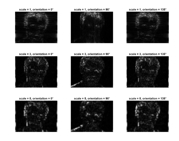
Each figure displays a grayscale image that represents the response of the wavelet at a specific scale and orientation to the input face image.

The brighter areas in the images represent parts of the face where the wavelet has a high response, indicating that the wavelet is well-matched to the local features of the image at that position.

• For small scales the visualizations will highlight fine details such as edges around the eyes, mouth, or nose
• At larger scales, the visualizations will emphasize more global structures, such as the outline of the face
• Different orientations will show directional features like vertical edges (e.g., the nose) or horizontal edges (e.g., eyebrows).

In practical applications, these extracted features are used in a machine learning model (e.g., SVM, Neural Networks) that can exploit the richer representation of the face respect to simple pixel values, leading to potentially more accurate recognition results.

Discrete Wavelet Transform (DWT) §

The Discrete Wavelet Transform (DWT) provides a discrete and compact representation of a signal in the time-frequency domain. Unlike the Continuous Wavelet Transform (CWT), the DWT operates with discrete parameters, making it more spacially efficient. The DWT handles scale and translation parameters differently.

Key Differences Between DWT and CWT §

The DWT is more spatially efficient compared to the CWT, using fewer coefficients to represent the signal.

Discretization:

• The CWT operates over a continuous range of scales and translations, requiring discretization for computational purposes (e.g., sampling).
• The DWT uses a discrete set of scales and translations, which are typically powers of two (dyadic scales and translations)

It’s also sometime called by mathematicians as logarithmical equispaced, but in CS is more common the dyadic.)

Signal Representation:

• The CWT provides a redundant, continuous representation of the signal.
• The DWT reduces redundancy by using discrete parameters, yielding a more compact representation with lower computational complexity.

Complexity:

• The computational complexity of the DWT is .
• The computational complexity of the CWT is

DWT achieves this by applying the hierarchical decomposition, breaking down the signal into approximation and detail at each level of decomposition.

Definition of the DWT §

Formally, the DWT of a vector in is the matrix:

• (n=discrete variable) is the discretization of the daugher wavelet (t=continuos variable) at scale and translation , which is defined as:

where is the mother wavelet.

Discretization §

The previous wavelet is continuos, (uses the variable t). Discretizing it in consists in choosing , , thereby expressed as:

Now compare it to the mother wavelet CWT:

Indeed, in DWT scales and translations are dyadic values

• (dyadic scale)
• (dyadic translatin)

In practice, the formal definition tells us that each entry of the matrix is expressed as the scalar (inner) product of with a scaled and translated (and discretized in time) version of the choosen mother wavelet .

Fast Wavelet Transform (FWT) Algorithm §

The previous definition is a formal definition, but more efficient implementation usually avoid this and uses the FWT Algorithm.

The FWT algorithm decomposes a signal iteratively into different level of approximation and detail coefficients.

Decomposition Levels §

The FWT operates through decomposition levels, with each iteration breaking the signal into two components:

• Approximation Coefficients Vector: represents the low-frequency components of the signal, capturing coarse information.
• Detail Coefficients Vector: represents the high-frequency components, capturing finer details of the signal.

After the first decomposition level, the algorithm refines its analysis by working only on the approximation coefficients obtainted from the previous step. This process continues iteratively, progressively isolating lower-frequency information and finer details.

Second decomposition and downsampling §

At the second decomposition level, the FWT operates only on the approximation coefficients computed in the first level. The length of the approximation is half of the length of the original signal, so what happens is a downsampling. In this step, again the FWT computes the two vectors: the approximation coefficients representing even lower frequencies and a new set of detail coefficients, which capture finer details but within a narrower and lower frequency band compared to the first level.

Final Decomposition §

At the final decomposition, the process ends when the approximation coefficients vector is reduced to a single component, representing the lowest frequency of the signal.

This component is analogous to the DC component in the Fourier series. Similarly, the highest-frequency details are isolated in the final detail coefficients vector.

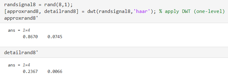
Application to random simple signal N=8 §

Let’s start using dwt on a simple random signal of length 8, using the Haar mother wavelet, just in order to look at the the approximation and detail coefficients of a single level decompostion

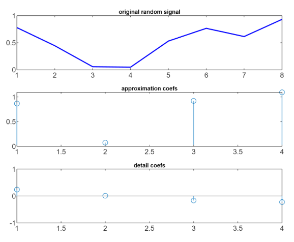
Note the different amplitude of the coefficients of the two vectors. (0,1 and -1,1 in the second part).

• The approximation vector captures the overall average trend, since it caputres the low frequency components of the signal
• The detail vector captures the high-frequency components, providing information about the small amplitude variations relative to the average trend.

Application to a randomly perturbated sum of two gaussian-modulated sines §

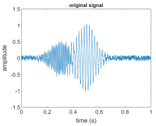
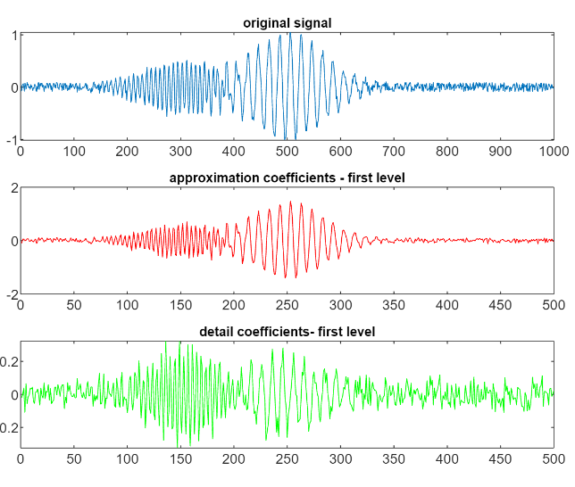Notice that the amplitude of the detail coefficients-first level is much smaller (-0.2 to 0.2).

For many types of signals, the bulk of the energy or important information content is found in these lower frequencies. Thus, approximation coefficients often contain the essential parts of the signal, such as the baseline melody in a piece of music or the main objects in an image.

Detail coefficients capture the high-frequency components, representing the fine-grained details within the signal. Detail coefficients often include noise, so by manipulating these coefficients it’s possible to remove noise while preserving important details of the signal.

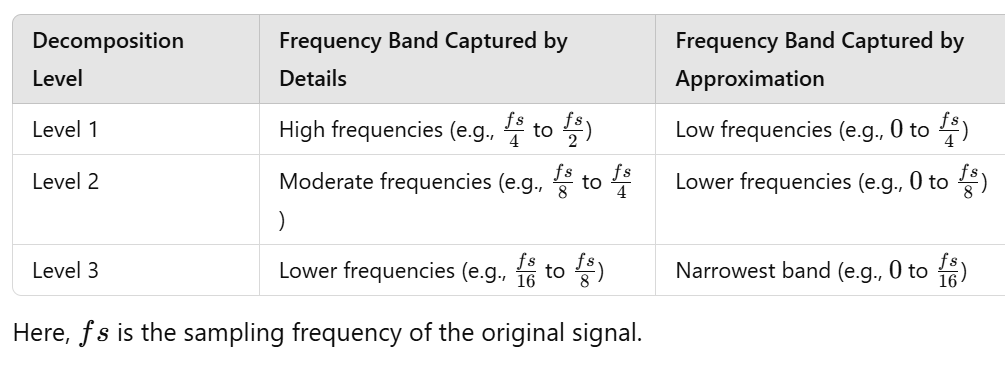
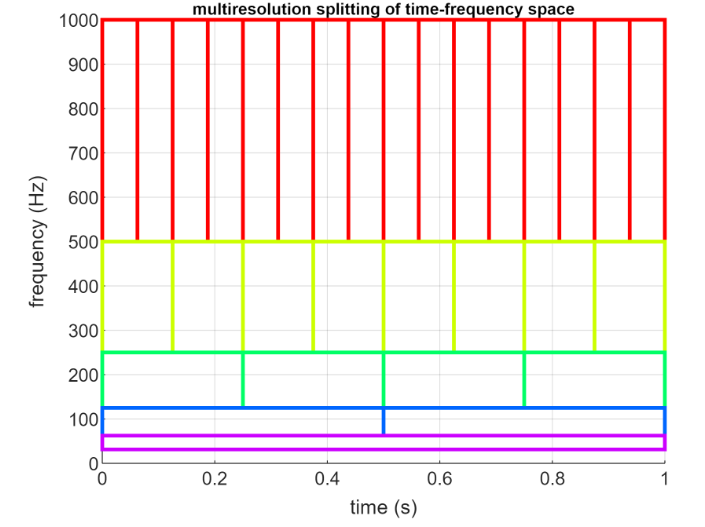
Frequency bands and octaves §

In order to clarify the idea of hierarchical multiresolution it is useful to introduce the concept of frequency band and octave.

Octave §

An octave referes to the interval between one frequency and its double. The term originates from music theory, where an octave represents the interval between one musical pitch (or musical note) and another with half or double its frequency.

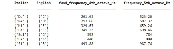
In a FWT algorithm, the signal is decomposed into frequency bands where each band (referred to as a level) covers an octave. This means each subsequent level of decomposition covers half the frequency range of the previous level.

In Fourier analysis, information in the time domain is distributed horizontally, while in the frequency domain, it is represented as vertical peaks.

When using the Short-Time Fourier Transform (STFT), you obtain a grid-like representation. However, this grid is uniform because the signal is not divided into separate components, unlike in wavelet-based methods.

Deeper insights into the computation of single-level decomposition §

Consider the example Application to random simple signal N=8.

We have the following matlab code: Each entry of approxrand8 consists of the sum of two consecutive samples from the original signal, weighted by a suitable value of the Haar wavelet. (Recall mother wavelets) So, approxrand8 has the following values:

While, detailrand8, consists of the difference between two consecutive samples weighted by a suitable value of the Haar wavelet, so it has the following values:

Recall that our signal has .

Haar mother wavelet and Haar sampling function §

The FWT algorithm applies a high-pass and low-pass filter to the signal.

• The high pass filter is derived from the discrete sampling of the mother wavelet function (Haar in our case)
• The low pass filter is derived from a discretization of the sampling function. The sampling function is uniquely associated to a wavelet. (Haar sampling function in our case)

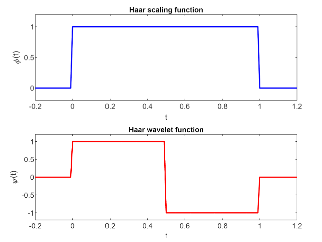
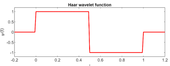
The Haar mother wavelet is

The Haar scaling function is a rectangular pulse

Discretization of the Haar mother wavelet §

To discretize in time our mother wavelet, we consider points given by the discretized daugher wavelets:

with

Since the signal has , downsampling the signal by 2 means that we have two vector of length 4, one for approximation and the other for details coefficients.

The signal is analyzed using 4 wavelet functions. For a single-level decomposition , and , putting these values in the previous formula we obtain:

for

The wavelet is nonzero if the argument of this function is between 0 and 1 (the support of the function), that is:

That is:

• or , Putting these constraints togheter:

Since , the wavelet spans just 2 time units (i.e. 2 indices).

Detail Coefficients §

The detail coefficients , are obtainted by means of the high-pass filter provided by the Haar wavelet:

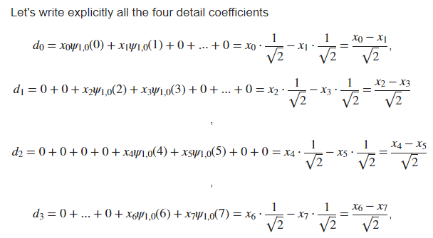More compactly we can write all four detail coefficients as:

Notice how the detail coefficients corresponds to the one we saw previously.

Scaling Functions §

This section is analogous to the previous one, but now we consider the scaling function :

We put and , and for discretization:

for

The scaling function is nonzero if Like before: or , . Thereby we get:

The approximation coefficients are obtainted by means of the low-pass filter provided by the scaling function:

In compact form:

Notice how the approximation coefficients corresponds to the one we saw previously.

Multiresolution framework §

We introduced the concept of hierarchical multiresolution analysis.

A multiresolution approach involves analyzing the input signal at various resolutions or scales. Each resolution, or decomposition level, corresponds to an octave band in terms of frequency content.

The algorithm remains largely the same, but it is applied iteratively across multiple levels. At each level, the process is performed on the approximation coefficients obtained from the previous level. In our earlier example, we considered a single level with . However, in a multiresolution approach, can take any value, with the scale defined as . Both low-pass and high-pass filters corresponding to the scaling functions:

and wavelet function:

respectively.

Mother Wavelets used in DWT and CWT §

DWT:

• Haar Wavelet and Daubecheis wavelets (including their variant)

CWT

• Morlet wavelet

The direct implementation of the DWT has a computational complexity of but using the FWT, this complexity is reduced to , making it linear with the number of samples.

This makes the FWT particularly suitable for real-time applications and the processing of large datasets.

Inverse DWT (or DWT Synthetis) §

The IDWT is defined as:

The ability to perfectly reconstruct the original signal from its wavelet coefficients is a key property for the use of DWT in real applications.

Fast IDWT §

It takes as input the approximation coefficients at the coarsest level and detail coefficients for every level, in decreasing order

Instead of downsampling, here we have an upsampling of the approximation coefficients at level and detail coefficients at level inserting zeros between consecutive entries of each of the two vectors.

Then the algorithm compute the convolution of:

• the upsampled approximation vector with a low-pass reconstruction filter (derived from the scaling function)
• the upsampled detail vector with a high-pass reconstruction filter (derived from the wavelet).

The sum of the two vectors obtained from these convolutions gives the reconstructed approximation vector at level . The process is iteratively repeated for each level.

At level the vector obtained is the reconstructed signal.

The time complexity is the same as FWT.

---