SC - Lezione 28 - Aliasing, Nyquist-Shannon Theorem, Fourier Transform

---

Domande, Keyword e Vocabulary §

• Aliasing
• temporal aliasing and spatial aliasing
• Nyquist-Shannon sampling theorem
• What is a bandlimited function?
• Nyquist rate
• Formula for reconstructing f(t)
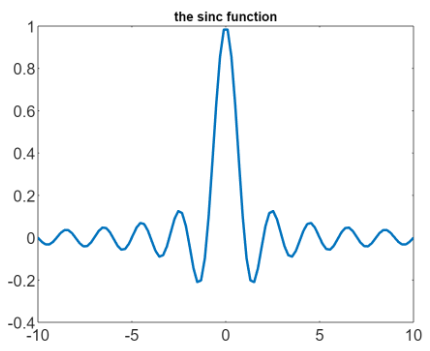
• sinc function
• Infinite Number of samples
• Demonstration of the Aliasing phenomenon
• Example: minimum number of samples for sampling correctly a signal
• Computing Nyquist rate, Sampling period, and Minimum Number of samples

Appunti SC - Lezione 28-29 §

Aliasing §

In the previous lesson we saw the Gibbs Phenomenon and how it depends from the FT.

Aliasing is a different problem that depends on the sampling.

Formally, two different continuos functions becomes indistinguishable after sampling. This leads to distortion during the reconstruction process, causing the reconstructed function to differ from the original. Aliasing can occur in both the time domain (temporal aliasing) and the spatial domain (spatial aliasing).

Nyquist-Shannon sampling theorem §

Let be a function that is bandlimited to , then can completely be reconstructed from a sequence of its samples where varies on all the integers and is the stepsize of the sampling, if and only if the sampling rate satisfies the following condition:

What is a bandlimited function? §

A function that contains only a finite range of frequencies . In practice, it’s a function whose variations are inherently smooth and do not exhibit abrut changes.

Nyquist rate §

When , then the sampling rate satisfies the minimum sampling rate

Formula for reconstructing f(t) §

The following formula is used:

Where

Is the normalized sinc function:

The Nyquist-Shannon theorem does NOT requires an infinite number of samples!

Demonstration of the phenomenon §

Consider a period of . Consider two complex waves:

defined on the interval .

Discretization: (Sampling) Consider a grid of equispaced points with stepsize . The sampled values of the two functions are and Substitute, with in the previous complex wave formula and we obtain:

where .

Then assume that , which can be rewritten as: and get:

Then by doing algebraic manipulation we get:

For the reason why see the root of unity definition.

The conseguence of the above formula is that, on the choosen grid of equispaced points, the two functions are not distinguishable.

Note that we get the same result if for any integer .

Simple example computing the minimum number of samples required for sampling correctly a signal §

Consider this function: on . The frequency is , so that the Nyquist rate is:

The corresponding sampling period, is obtainted by the inverse of :

How to compute the Nyquist rate §

Consider of the form , is the angular frequency (See recap of the elements of a signal)

The fundamental frequency in cycles per unit time is related to the angular frequency by this formula:

for this becomes:

cycles per unit time. The Nyquist rate is obtainted as twice the maximum frequency present in the signal, so:

How to compute the minimum number of samples §

• the interval length is ;

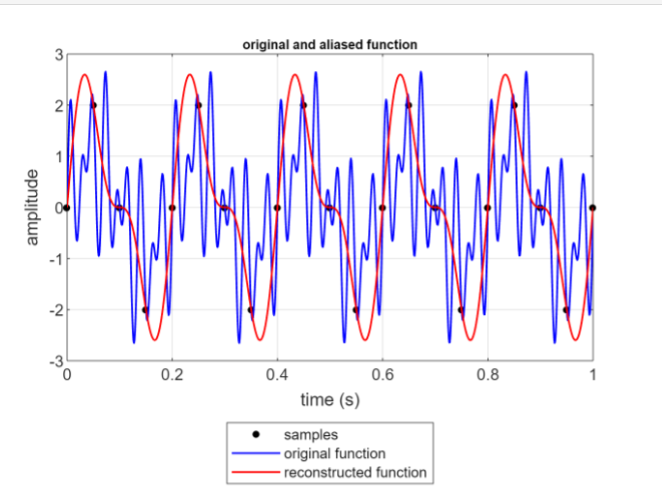
Conseguences of choosing an insufficient number of samplings §

If we choose then we have a wrong reconstruction.

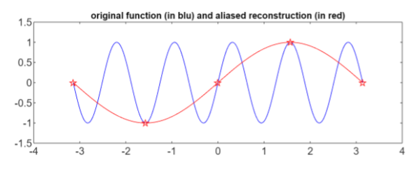We observe that the aliased reconstruction in red is that has a frequency . This happens because the number of samples is insufficient to represent the highest frequencies of the signal accurately.

The reconstruction gives a function of frequency:

• in the example N=4

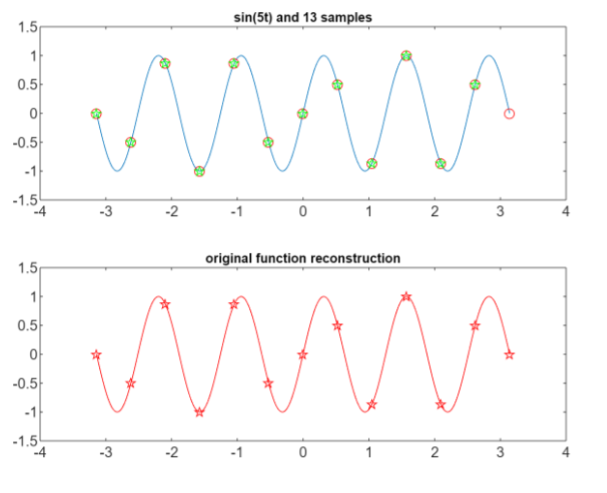
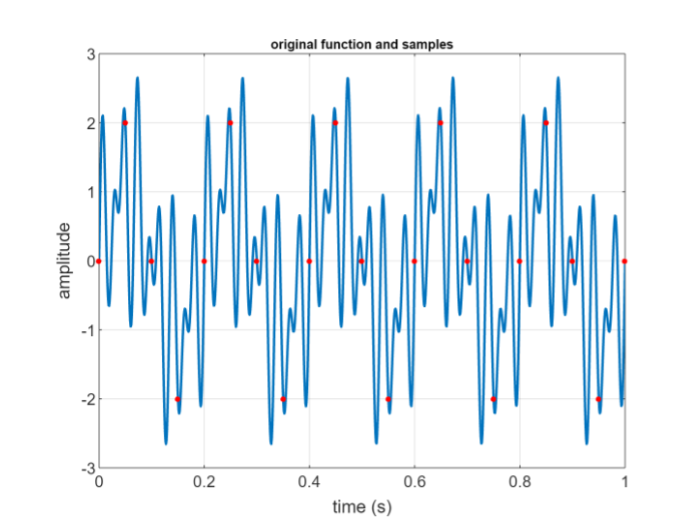
Ofcourse, this doesn’t happens when is sufficiently large:

More complex example of what happens when a function is sampled below the Nyquist rate §

Consider the function:

This function combines multiple sine waves of different frequencies:

• and the Nyquist rate is:

For convenience, since for example a component of the signal then the corresponding sampling frequency would be:

then we have that is easily computed and we represent it in Heartz for second.

Suppose that the sampling rate is set to Hz Hz which causes aliasing, where higher frequencies fold back into lower frequencies.

We need to compute that are the frequencies aliased

Since and are both higher than the sampling rate we choose, they will be folded into the frequency interval of the frequencies that can be reconstructed with the sampling rate .

Nyquist frequency §

the frequency

is called the Nyquist Frequency (not to be confused with that is the nyquist rate).

The relationship between aliasing and the Nyquist frequency is the following: If is the choosen frequency, it will be aliased in the frequency: where is an integer such that .

Back to our example: only will be correctly reconstructed. and will give rise to the aliased frequencies and that since are given by:

Relationship between Nyquist frequency and Nyquist Rate §

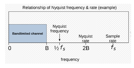
• Nyquist rate : 2 times the highest frequency (bandwidth); it’s a property of the function (a continuos-time signal)
• Nyquist frequency : half the sampling rate; it’s a property of the sampled function (a discrete-time digitized sound)

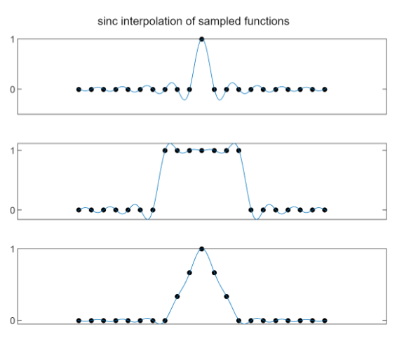
The Sinc Function §

Property of the Sinc Function §

It can be used for reconstruct any bandilimite function through Lagrange interpolation of a set of sampled values on an equispaced grid:

• is a stepsize on the grid

The sinc interpolation of a function is called cardinal interpolation, meaning that the weights of the interpolation formula are the samples themselves.

Convolution: the above formula can be seen as the convolution of the sampled function and the kernel .

Choosing : if is too large then there will be a distortion of the reconstruction. This interpolation works well when ( is the sampling period).

Fourier Transform §

The inverse is:

We used the circular frequency but we could also have used the angular frequency by substituing

Dirac Delta §

is the Diract delta function, which is defined as:

It’s not a function in the traditional sense but a generalized function. It has the following key properties:

• unit area: the integral is 1: despite his infinite height
• sifting property: it can sift out the value of a function at a specific point

The FT of is the constant function , meaning that is NOT band limited and contains all frequencies at same amplitude.

Properties of the Fourier Transform §

• is a linear operator: is
• The FT of is

Convolution §

The FT of a continuos convolution of two functions: is .

For continuos functions, the convolution is defined as:

While, when we saw the discrete convolution, we saw it used the summation

Another related property of the FT is that: equals to i.e the continuos convolution of and

Derivative §

The FT of is . In general, the FT of is

Duality §

if the FT of is , then the FT of is

Bandlimited function §

If the FT of has a finite support, then is a bandlimited function (its frequency content is the support of its FT).

Parseval theorem §

Recall that this also holds in the discrete case.

Example §

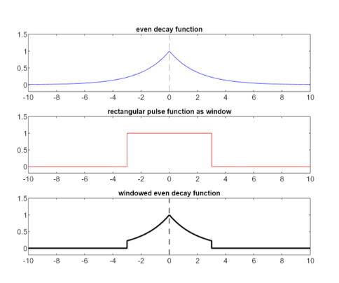
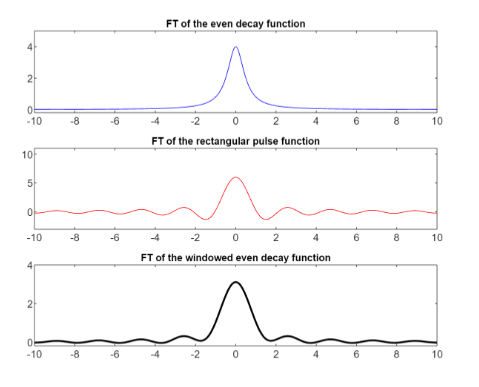
• The even decay function defined as: restricted in the finite interval
• The even rectangular function we call , of half-length
• The “windowed even decay function” is obtainted by convoluting the two functions in the frequency domain: is equivalent to

In the frequency domain:

How to compute the Fourier Transform §

The algorithm is similar to the one designed for approximating Fourier Coefficients and partial sums of a Fourier Series.

This algorithm only approximate the value of the FT of a function, since it would be impossible or too costly to compute the entire function.

Given ( is choosen as even number) equispaced samples: in a limited interval . The algorithm computes the approximations: in

The main steps of the algorithm for the FT are:

• define the vector of samples such that ,
• Compute the DFT of
• Reorder the vector
• Append a copy of the first component a the end and multiply all entries by the scaling factors: , for
• Compute the frequency ,

What's the difference with the algorithm for computing the FS?

With respect to the fourier series algorithm, here we have an extra step at the end: compute the frequency ,

A glimpse to Fourier series and Transform in Functional Analysis §

Hilbert Space in and Fourier Series §

Consider a space of functions that possess the property that i.e the so called Hilbert space .

The previous identity define the norm of a function

The inner scalar product between two function is defined as: . Notice how the definition is similar to the norm of a function.

Now consider the functions: for . (functions, plural because for each , it’s a different function). These functions forms an orthonormal basis for the space since:

for (because defines the inner product and it is 1)

Now consider the Fourier coefficients of a periodic function in . These are the components of onto the orthonormal basis , in fact we could write in this notation:

following this point of view, the Fourier Series of is the orthogonal projection of on the space spanned by this basis. (the subspace of periodic functions in )

Hilbert Space in and Fourier Transform §

Now consider the space of functions that possess the property that: i.e the so called Hilbert space .

This identity define the -norm of a function . The inner scalar product between two functions in is defined as:

Consider the functions for , they form a continuos basis for the space . But unlike the previous [[#Hilbert Space in |case]], here represents a continuos variable corresponding to frequency, and we have non-periodic functions.

They form an orthogonal basis, since it can be shown that: for

The FT of a function can be viewed as the projection of onto a continuos orthogonal basis of the space , specifically using the basis of complex exponential functions for .

---