SC - Lezione 31 - 2D DWT and its inverse, JPEG2000, High-pass and Low-pass filters in the Time domain

---

SC - Lezione 31 §

---

Checklist §

Checklist

Domande, Keyword e Vocabulary §

• DWT Application: denoising a signal
• Median Absolute Deviation
• Universal Threshold
• 2D-DWT and its inverse
• Matrix G
• rows and columns
• Single Level 2D-DWT steps
• LL, HL, LH, HH matrices
• approximation, horizontal, vertical, diagonal details
• Time Complexity of the 2D DWT
• Inverse 2D-DWT
• JPEG2000 Image Compression Algorithm
• CWT vs DWT time complexity
• CWT and DWT in Functional Analysis
• Orthogonal basis vs Overcomplete dictionary
• CWT as series of inner product in functional analysis
• DWT/FWT as linear operator
• Heisenberg Uncertainity
• Real-world examples of signal processing
• High-pass and low-pass filters in time domain
• Impulse response
• Ideal low/High pass filter
• Finite Impulse Response Filter
• Hamming window
• Band-pass filter

Appunti SC - Lezione 31 §

DWT Application: denoising a signal §

We consider a signal and we apply some noise to it

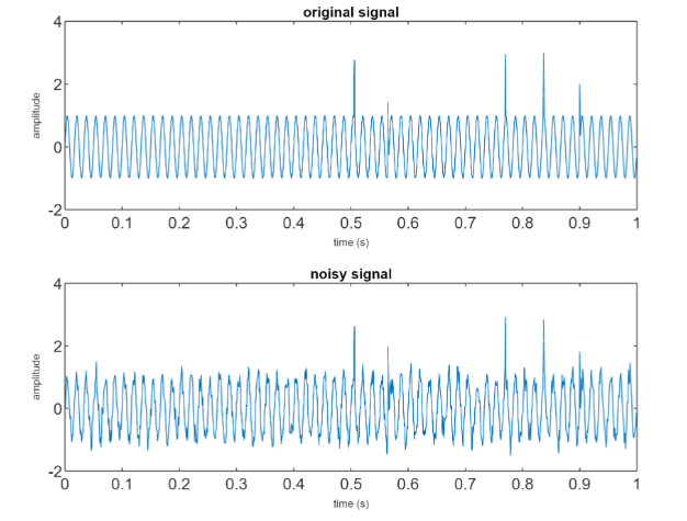
We use “transient spikes” since it’s a non-stationary noise. We apply the CWT up to the 4 decomposition level.

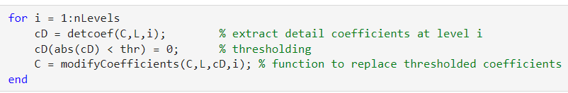
Then we need to estimate the noise level, that is the standard deviation of the noise of the signal. Since the highest-frequency detail coefficients are dominated by noise, which is often assumed to be Gaussian, we use the detail coefficients of the first decomposition level.

A reliable estimate of the standard devitation is based on the Median Absolute Deviation (MAD) that is: MAD() = median() and gives:

The threshold is commonly chosen as the so-called universal threshold given by: where is the length of the signal.

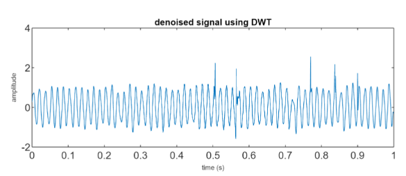
Then, to apply the denoise we set any entry below that threshold, in the detail vectors, to 0 :

2D-DWT and its inverse §

The 2D-DWT involves the multiple use of the DWT in two directions.

The matrix G that represent our signal is decomposed into multiple levels of detail and approximation. If the has rows and columns, the output of a single-level 2D DWT are four matrices of size:

Single level 2D-DWT §

The steps are the following: first an horizontal transformation is applied and is splitted intwo two matrices. Then a vertical transformation is applied on the two matrices, resulting in 4 matrices.

The matrices after the horizontal transformation: 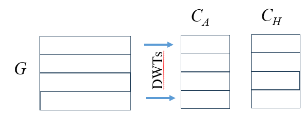They are vectors of coefficients for each row, that are just stored as a horizontal approximation coefficients that we call and

Then, in the vertical transformation: 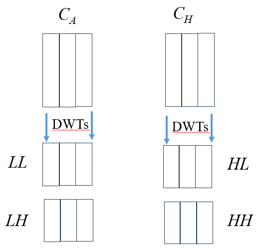We apply the DWT again to each vector, obtaining ,, and

This process and be mathematicall represented as follows for a single level decomposition:

• approximation (Low-Low, ): result from applying low-pass filters in both horizontal and vertical directions. They capture the smooth parts of the image without rapid intensity changes
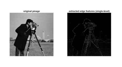
• horizontal detail (High-Low, ): result from applying a high-pass filter horizontally and a low-pass filter vertically. They capture horizontal details or edges
• vertical detail (Low-High, LH): result from applying a low-pass filter horizontally and a high-pass filter vertically. They capture vertical details or edges
• diagonal detail (High-High, HH): result from applying high-pass filters in both directions. They capture the high-frequency content that often corresponds to changes or features oriented diagonally, i.e. both horizontally and vertically.

Time Complexity §

as we expect it’s similar to the 1D DWT complexity.

Inverse 2D-DWT §

Reconstruct the original image from four matrices .

The algorithm can be summarized in:

• upsampling the four matrices
• Convolution along the rows of and with a low-pass reconstruction filter
• Convolution along the rows of and with a high-pass reconstruction filter
• Sum the filtered outputs from and to form an intermediate horizontal approximation
• Do the same with and for an intermediate horizontal detail
• Upsample again the columns of the two intermediate matrices
• Convolve the columns of the intermediate approximation matrix with the low-pass reconstruction filter
• Convolve the columns of the intermediate detail matrix with the high-pass filter
• Add the filtered outputs from both convolutions to reconstruct the original signal Time Complexity is the same.

JPEG2000 - Image compression algorithm §

JPEG2000 is a standard for image compression that significantly improves over its predecessor JPEG, it uses the FWT. It can apply both lossless and lossy compression.

How the algorithm works §

• Preprocessing: the image is preprocessed, for instance the image could be divided into smaller blocks and a color space transformation could be applied
• 2D-DWT: apply the transformation as we saw in this lesson, we obtain 4 subbands matrices
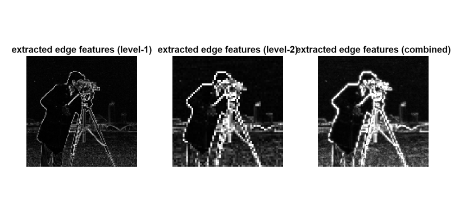
• Subsequent Decomposition: the matrix (that represents the coarse approximation of the image) is further decomposed into subsequent levels, progressively extracting finer details
• Quantization: the wavelet coefficients are then quantized. In lossy compression, this step significantly reduces the amount of data by approximating the coefficients to a lower precision;
• Entropy coding: the quantized coefficients are then encoded using entropy coding techniques which further compresses the data by exploiting the statistical properties of the coefficients; (We dont’ go in deep with this)
• Post-processing: the encoded data are organized into a codestream ready to be stored or transmitted

Matlab simplified code example §

We discuss a simple educational Matlab code that demonstrate a basic implementaton of JPEG2000-like compression using 2D-DWT

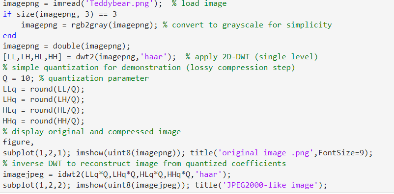
The core step is quantization. By dividing the wavelet coefficients by a quantization parameter , rounding them to integer, and then multiplying back by for reconstruction, the code simulates a lossy compression process.

CWT vs DWT - Time complexity §

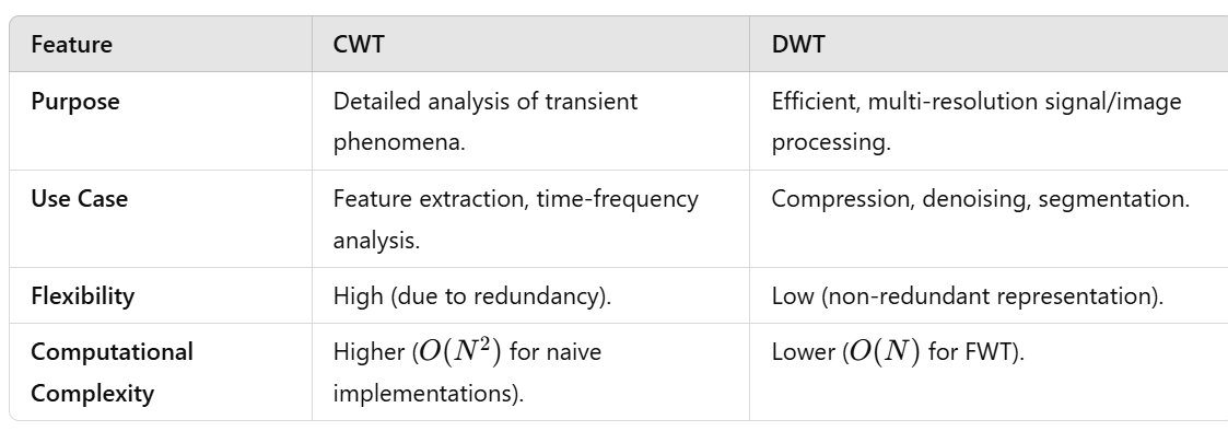The choice between DWT and CWT depends on the application requirements.

If one needs a highly detailed analysis where the exact scale and position of signal features are crucial, CWT might be the better choice despite its higher computational cost.

On the other hand, if one requires efficient computation and storage, especially for tasks like image compression, denoising, or when working with large datasets, DWT’s discrete and compact representation offers significant advantages.

A glimpse to CWT and DWT in Functional Analysis §

See also: A glimpse to Fourier series and Transform in Functional Analysis

Unlike the FT, where sines and cosines form an orthogonal basis in , in general wavelet functions do not always from and orthogonal basis.

There are notable exceptions, such as the Haar wavelet and certain Daubechies wavelets, which are designed to form orthogonal bases.

A wavelet family forms an overcomplete dictionary for meaning it provides a redundant set of functions for representing the original function

Orthogonal basis vs Overcomplete dictionary §

An orthogonal basis is a set of vector, orthogonal to each other, that allow the unique, efficient, and non-redundant representation of every element in a vector space.

An overcomplete dictionary is a set of vector (or functions) that is used to represent elements in a vector space, but it contains more vector than necessary to span the space (that’s why we say it’s redundant). This imply that the same vector can be represented in multiple (in fact infinite) ways.

CWT vs DWT and orthogonal wavelets §

• CWT prefers non-orthogonal wavelets for flexibility and redundancy
• DWT uses orthogonal and compactly supported wavelets.

CWT as series of inner product §

CWT is a linear operator from into a space of functions of two variables: -

Consider the CWT:

In , the norm of a function is:

Parseval-like theorem for CWT §

We can use the previous formula to express a Parseval-like theorem for CWT as:

• is a proprtional factor that depends from the chosen wavelet

DWT/FWT as linear operator §

It can be shown that the DWT/FWT is a linear operator from onto (that is a matrix), transforming the input signal vector in a vector containing the approximation and detail coefficients.

where is the FWT matrix, representing the wavelet basis functions.

As we said, some wavelets are orthogonal, therefore

It can be shown that the overall multi-level DWT (multiresolution) can be tought of as applying a sequence of orthogonal transformations to the input vector, and the entire process can still be represented by an orthogonal matrix.

Heisenberg Uncertainity Principle §

This principle imposes a theoretical limit on how precisely we can localize a signal simultaneously in both the time and frequency domain. This limit applies to all time-frequency analysis methods that we saw (FT included).

More formally:

• is the uncertainity in time
• is the uncertainity in frequency

It’s impossible to arbitrarily reduce uncertainty in both the time and frequency domains simulanteously.

From real-time analysis to intelligent insights: integrating signal processing and AI §

As real-world examples, we can consider Biomedical signal processing and Vibration analysis in industry.

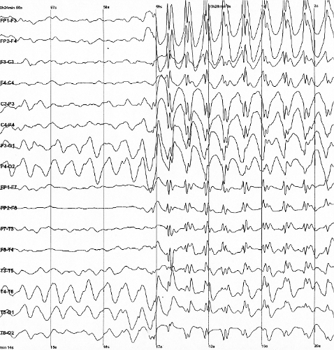
Electroencephalogram (EEG) devices or Electrocardiogram (ECG) monitors often include embedded FFT analysis to provide real-time frequency information about brainwaves or heart rhythms. As second step, techniques like STFT or wavelet transforms are used to analyze non-stationary components, such as detecting epileptic seizures or arrhythmias. As a further step, Machine learning/AI algorithms are applied to classify different signal patterns (e.g., identifying neurological disorders or predicting cardiac events).

Vibration sensors or accelerometers in machinery (e.g., for predictive maintenance) embed FFT analysis to monitor frequency components of vibrations. Advanced analysis using CWT or DWT helps identify transient phenomena, like the early onset of bearing failures or gear faults. As last step, AI-based predictive models analyze patterns over time to forecast equipment failure and optimize maintenance schedules. accelerometer_cross_section.webp

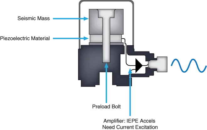
High-pass and Low-pass filters in the time-domain §

We have discussed DFT,FT,CWT and DWT to filter out specific frequencies from a signal.

However, designing and applying filters, such as low-pass or high-pass filters, does not inherently require any of the previous technique.

Filters can be designed and implemented directly in the time domain using their “impulse response”. Then the effect of the filter is realized through convolution of the signal with the impulse response.

Recall that the impulse response is the output signal that results when an impulse is given as input to the filter.

low-pass and high-pass filters are used for example for the efficient implementation of the DWT.

If is an input function, the output is obtainted through convolution of the function with the filter’s impulse response:

by the superposition property, the system response to can be expressed as the weighted sum of the responses to each shifted impulse, so that the time-shifted impulse response to is

Low pass filter §

Ideal low pass filter: passes all frequencies below a cutoff frequency and completely attenuates all frequencies above :

In the time domain, the impulse response is the Inverse Fourier Transform of its frequency response .

The ideal low pass filter is a rectangular function. Its inverse is a sinc function: where is the normalized cutoff frequency. For example, if a signal is sampled at , the nyquist frequency is .

A low pass filter designted with a cutoff frequency of would have a normalized cutoff frequency of that is .

Constructing an ideal, infinite, low pass filter is impractical

Finite Impulse Response Filter (Low-Pass) §

A window function is used to truncate the sinc function and gradually reduce its amplitude towards the edge.

For example let’s see the Hamming window:

• is the total width of the window in time. By sampling this continuos function at specific time intervals, we obtain the discrete version.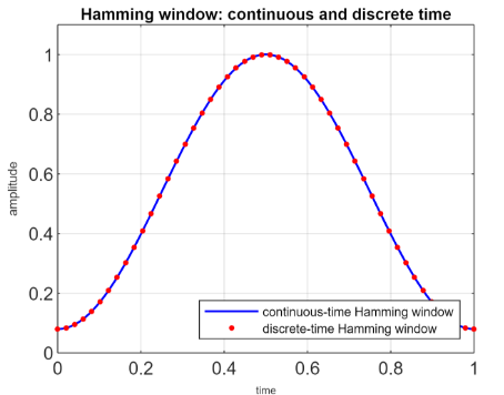

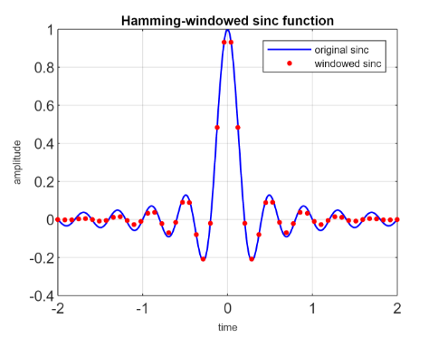
The impulse response of the FIR low-pass filter is:

High pass filter §

Ideal High-pass filter §

This ideal filter passess all frequencies above a cutoff frequency and attenuates those below

The filter could also be expressed as

The time-domain impulse response is the IFT of the frequency response and remembering that the inverse FT of the constant 1 is the Diract delta functions we have that:

This technique of expressing an high-pass filter as inverted low-pass filter is called spectral inversion.

The impulse response of the FIR high-pass filter is: .

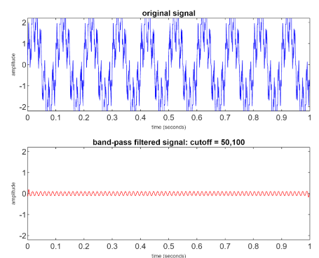
Band-pass filter §

A band-pass filter is a filter that allows signals within a specific range of frequencies (the “band”) to pass through while attenuating frequencies outside this range. It combines the effects of both a high-pass filter (removing frequencies below a lower cutoff) and a low-pass filter (removing frequencies above an upper cutoff).

We may construct this filter using an approach known as filter cascading or filter stacking. In essence, the high-pass filter is sequentially applied to the input signal to remove low-frequency component. Then we do the same thing with the low-pass filter to remove high frequency components.

---