SC - Lezione 27
Checklist
Domande, Keyword e Vocabulary
- Fourier Series (FS)
- Fourier Coefficients
- FS in complex form
- Periodic function
- sum of sines and cosines
- real coefficients of the Fourier Series
- Relationships between real coefficients
- Review of terminology of trigonometric functions: amplitude, phase, initial phase, circular and angular frequency and period
- Properties of Fourier Coefficients
- Parseval Theorem and energy of a function
- Trigonometric polynomial
- Discintinuos functions and Gibbs phenomenon
- Convergence of the fourier series
Appunti SC - Lezione 27
Fourier Series (FS)
The Fourier Series represents a periodic function (sin, cosin) as an infinite sequence of Fourier coefficients. These coefficients capture the function’s frequency components.
The
is a periodic function; : the period of , satisfying recall for all ;
Fourier Series in complex form
Using the Fourier coefficients, the periodic function can be reconstructed as:
This converts the infinite sequence of Fourier coefficients into a periodic function.
Alternative expression of the Fourier Series
Using the Euler’s formula:
- We consider a period
over the interval is expressed as infinite sum of cosines and sines defined over the previous interval and are called real coefficients and have a particular definition:
and
Using the Euler’s formula and considering this interval
- The exponential is:
Relationship between real coefficients
for for
Conversely, to find
for for
Review of terminology of trigometric functions
A function
amplitude phase initial phase circular frequency (number of complete cycles or oscillations, measured in Hz)
- Angular frequency:
(rate of change of angle, measured in radiants per time units) i.e you can write - Period:
Approfondimenti
Application of the FS: draw an elephant
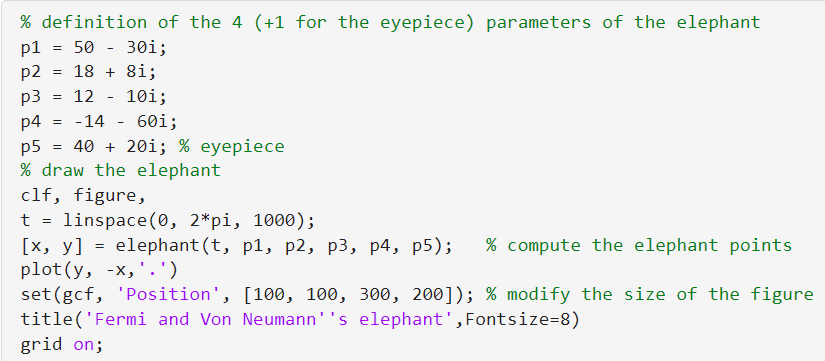
- p1,p2,p3 and p4 draws the elephant body, p5 is the eyepiece
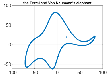 This example shows that any function can be reconstructed using an appropriate parameters.
Properties of Fourier Coefficients
Even, odd and real valued function
- if
is an even function then for all (the FS contains only cosines) - if
is an odd function then for all (the FS contains only sines) - if
is a real valued function, then for all
Parseval Theorem (Energy of the function)
The energy of the function
Energy of a function
The term energy comes from physics, where
represents the power density (in an electrical or acoustic signal) The Parseval’s theorem confirm that energy is conserved between the time and frequency domain.
Trigonometric polynomial
A trigonometric polynomial is a partial sum of a Fourier series. In practical applications, it is not feasible to consider an infinite number of coefficients, so we typically limit the series to
The
is even, resulting in coefficients .
The coefficients can be written also in complex form as:
Example: computing the Fourier Coefficients (FC)
We consider the function 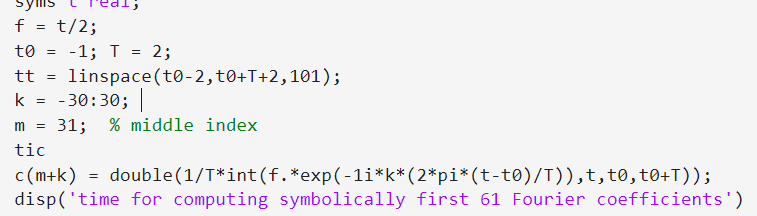 Note that the period is fixed to
Using the complex coefficients calculated exactly, we evaluate the first 30 partial sums of the Fourier series over the interval 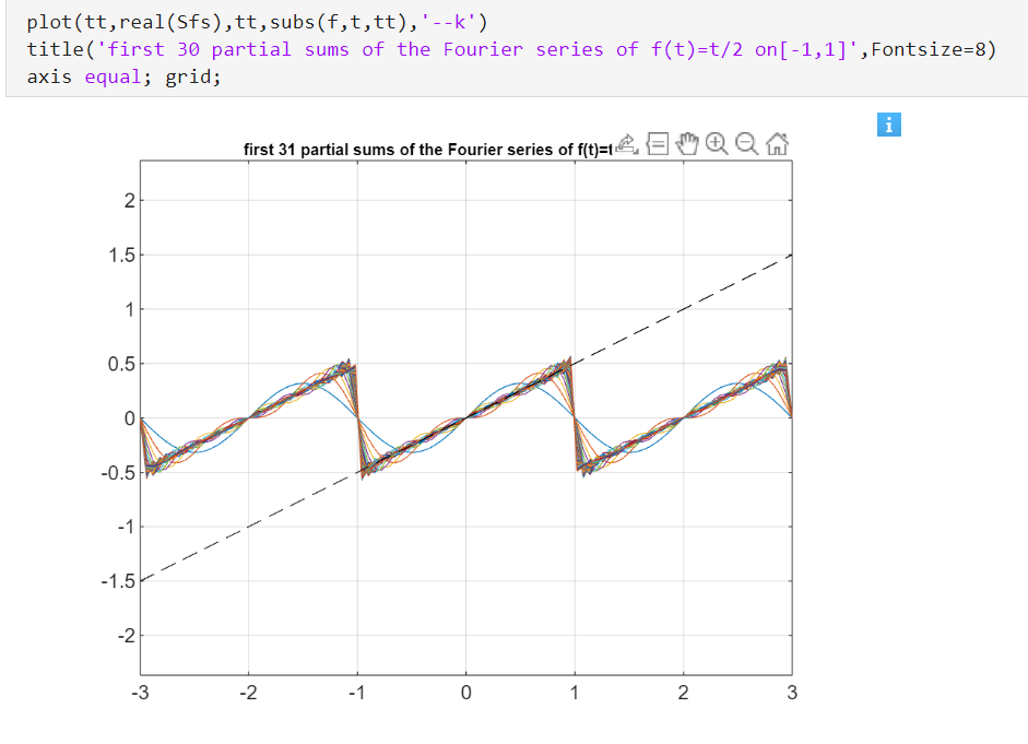 We fixed (in the matlab code) T=2, so the partial sums of the Fourier Series are periodic approximation of period
The functions generated by the partial sums of the FS extend periodically
Discontinuos functions and Gibbs phenomenon
Formally, a function is not defined at a point of discontinuity (jump point). Logically, we expect the value at such a point to be the midpoint between the left-hand limit and the right-hand limit.
This is evident in the previous example: at x=1, the value is 0, which is the midpoint between 0.5 (left-hand limit) and −0.5 (right-hand limit).
Convergence of the FS:
The FS converges pointwise at
is continuos at the interval has a finite number of discontinuities within the period
Then, the FS converges uniformely in any interval where
Near a jump discontinuity, the FS exhibits oscillatory behavior called Gibbs phenomenon.
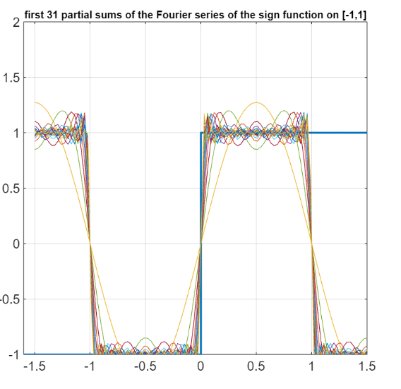
We use 31 partial sums, but even with more terms, the error does not vanish; instead, it approaches a limit of about 9% of the size of the jump. This behavior is independent of sampling, as we are directly working with the Fourier Series, not sampling the function.
(Favorite question at the exam) We emphasize that the Gibbs phenomenon occurs even without sampling, when attempting to reconstruct or approximate a discontinuous function using a finite number of exact terms from its Fourier series. This is obvious, as we are trying to approximate an infinite function with a finite number of terms.
How to compute Fourier Coefficients
Using the symbolic computation of Fourier Coefficients is very costly and not suitable for large scale application.
One possible approach is using numerical integration (quadrature algorithm) but this numerical problem is unstable when the function has singularities.
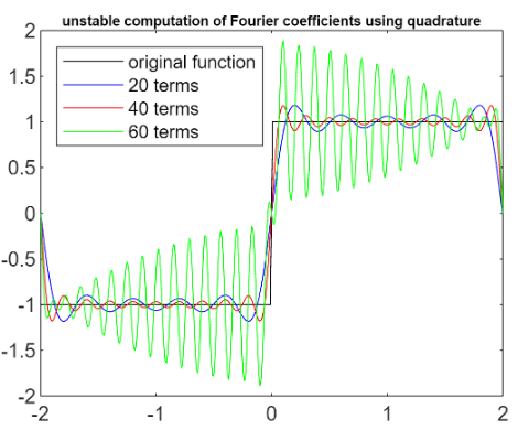
The best way is to use the DFT/FFT to approximate simultaneously all the coefficients of a partial sum of a Fourier Series.
By means of DFT we can simultaneously approximate all the coefficients of a partial sum of a Fourier Series. This algorithm can be derived from the trapoezoidal rule.
Trapezoidal Rule
Recall that the trapezoidal rule is used in integration theory (recap youtube video here)
Consider a trapoezoidal quadrature rule on
First notice that, since the periodicity of the DFT,
- we have the sum of the most left point (evalued at -T/2) and the most right point evalued at (T/2) divided by two
- Then we have the summation of all the internal point (
goes from to )
- the exponential is put outside of the parthentesis (messo in evidenza), to do this we first have to multiply the most right term by 2 this because:
(raising algebraic properties)
note also that:
Trapezoidal rule in exponential form
We can write in exponential form
where:
this is quite similar to the DFT except for the range of the index and the factor in front of the summation.
Comparison of the DFT formula and the trepzoidal rule in exponential form
If we consider a new index
the index
Express the DFT as trapezoidal rule
We can express the DFT of the vector
for corresponds to for for corresponds to for
With this approach, the DC component is positioned in the middle, flanked by negative frequencies on the left and positive frequencies on the right.
Approximating Fourier Cofficients - Algorithm
In summary the main steps of the algorithms are:
- define the sample vector
- compute the DFT
of - rearrange the vector
by shifting the zero-frequency component to the center - append a copy of the first component of
at the end - multiply each component by the scale factors
, .
The fftshift function in matlab effetuate the shift of the direct current component at the center of the vector.
Approximating Fourier Series - Algorithm
Conversely the approximation of the values of a partial sum of a Fourier Series on a grid can be efficiently computed using the IDFT/IFFT. In this problem the inputs are
The main steps of this algorithm are
- define the sample vector
- change the sign to alternating components of
- rearrange the vector
by shifting the zero-frequency component to the center - compute the Inverse DFT
of - append a copy of the first component of
at the end, and multiply all components by the scale factor
In the next lesson we will see Aliasing. Another important thing to remember for the exame is that while the GIbbs phenomenon it’s a problem of the Fourier Series, the Aliasing is a problem that depends from sampling and frequency.