SC - Lezione 29
Checklist
Domande, Keyword e Vocabulary
- Wavelet
- Continuos Wavelet Transform of a signal definition
- Scale and Translation
- Mother Wavelet
- Comparison of different wavelets
- Gabor Function
- Morlet wavelet
- Effects of scale and translation
- How to compute the CWT
- Scalogram
- Linear Scales vs. Logarithmic Scales
- Time complexity of the CWT
- Matlab cwt function
- Matrix of the wavelet coefficients
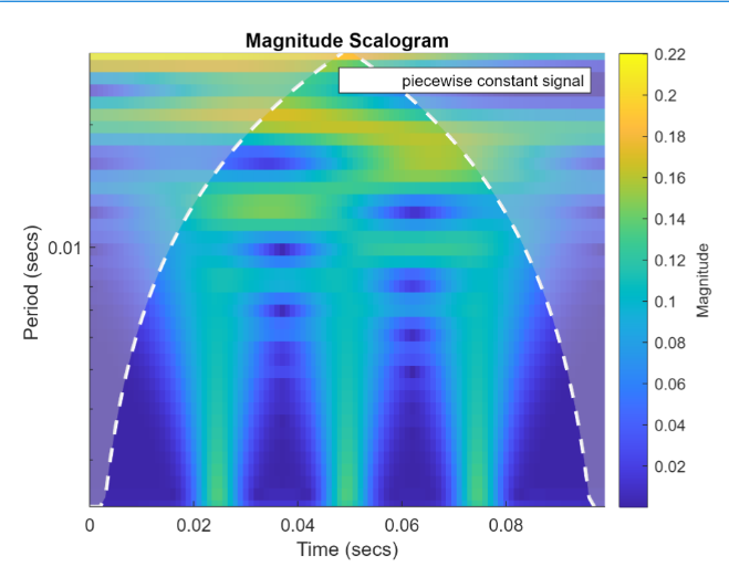
- Parts of a Magnitude Scalogram
- Inverse Continuos Wavelet Transform
Appunti SC - Lezione 29
In this and the following lessons we will see the CWT and DWT, that are advanced tools for time-frequency analysis.
Recall that we studied the Short-Time Fourier Transform, that is a fourier transform that uses a window size in the time domain. The STFT has a limitation regarding the window size that is fixed.
The CWT and DWT introduce a new analysis tool called wavelets
Continuous Wavelet Transform (CWT)
Wavelets
It’s a function that represents a small, localized wave with its energy concentration time.
A difference between wavelet and sinusoidal functions of the Fourier Analysis is that wavelet are localized both in time and frequency. Sinusoidal functions lacks time localization, thus it’s not that great for non-stationary signals where components change over time.
CWT
CWT is a tool that decompose a signal into wavelets.
The CWT of a signal
is the mother wavelet is the scale is the translation (or shift) denotes the complex conjugate of
Another way to see the above function is the continuos convolution of the function
Scale and translation - part 1
- scale
is inversely related to the frequency of the wavelet; - smaller scales corresponds to compressed wavelets (high-frequency and small time interval)
- viceversa, larger scales corresponds to stretched wavelets (low-frequency and large time interval)
- translation
shifts the wavelet along the time axis, allowing the analysis of different time segments of the signal;
Mother Wavelet
A mother wavelet is a prototype function that is used to generate a family of wavelets (called daugher wavelets) thrugh scaling and translation. It is often well-localized both in time and frequency domains, has a finite support (see support of a function), or rapidly decaying outside a certain range.
A mother wavelet must have certain properties:
- zero average: the integral of the mother wavelet, over the entire domain, must be zero. This property allows the wavelet to measure changes in a signal rather than its average value.
- finite energy and normalization: the total energy of the wavelet, scaled across all possible scales, is 1.
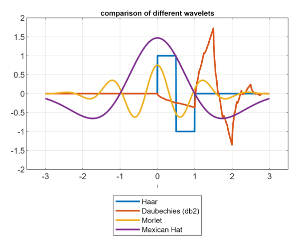
- Haar wavelet: constant real piecewise function with values
, otherwise 0 - Daubechies wavelet: real, maximal number of vanishing moments for some given finite support
- Morlet wavelet: defined by a plane wave modulated by a gaussian window, it has infinite support.
- Mexican Hat: real, minus second derivative of the gaussian function.
Gabor function and Morlet wavelet
In order to show a function that describes an oscillation eveloped in a localized impulse, we introduce the Gabor function.
The Gabor Function:
- t is the time or spatial variable
is the frequency of the sinusoidal is the standard deviation of the Gaussian evelope, controlling the window width. 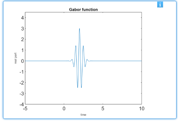
To apply the Gabor transform to a signal
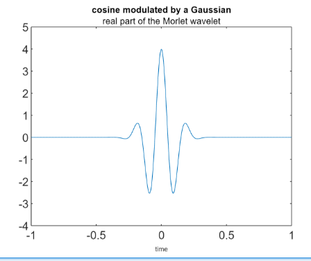
Now we consider a cosine wave, modulated by a Gaussian, to define the real part of the Morlet wavelet, which is strictly related to the Gabor function:
is a normalization factor is the standard deviation is the frequency of the cosine function
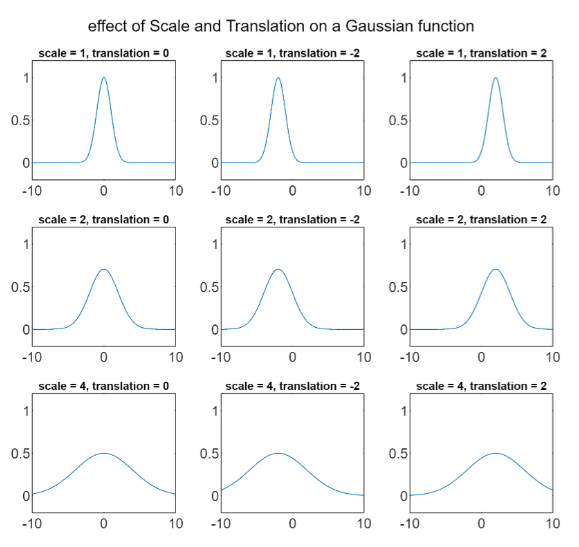
Scale and translation - part 2
Let’s see what are the effect of scale and translation.
The scale controls the frequency range that the wavelet can capture. Increasing the scale allows the wavelet to capture lower frequency components, while decreasing the scale allows it to focus on higher frequency components
As the scale changes, also the wavelet width in the time domain changes: larger scales make the wavelet wider in time, while smaller scales make it narrower
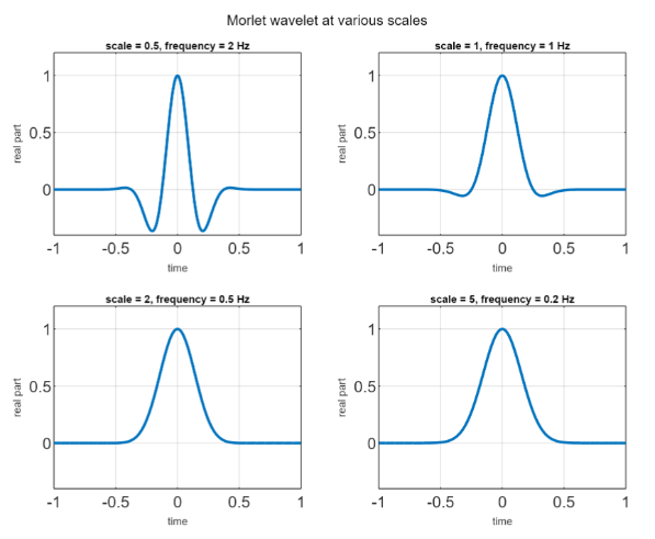
Conversely, the translation parameter shifts the wavelet along the time axis, enabling precise localization of features within different time intervals of the signal.
Scale and energy: since there is a normalization factor
How to compute the CWT
The Algorithm for computing the CWT of a function
The algorithm also computes and display the scalogram of
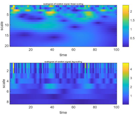
Scalogram
A scalogram is a visual representation of the CWT of a signal, showing how the frequency content of the signal varies over time.
It is generated by plotting the squared magnitude of the wavelet coefficients, as a function of both time and frequency (or scale).
Scalogram vs Spectogram: we saw spectogram in the context of the STFT. Both are visual representation of how the frequency content of a signal varies over time, but they are derived from different type of analysis.
Linear Scales vs. Logarithmic Scales
You can use either linear or logarithmic scales, depending on the nature of the signal:
- Linear Scale: Frequencies are evenly spaced, such as from 1 to 20. This scale is best suited for signals with a uniform frequency distribution. It provides consistent resolution across the entire range of frequencies.
- Logarithmic Scale: Frequencies decrease exponentially, covering a wider range. This scale offers higher resolution at lower frequencies, making it ideal for analyzing signals with details that span across a broad range of frequencies.
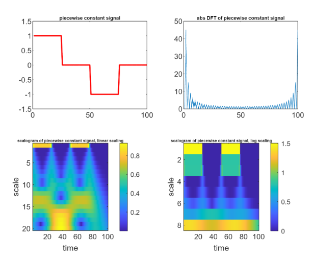
 Another example:
Time complexity
For a signal of length
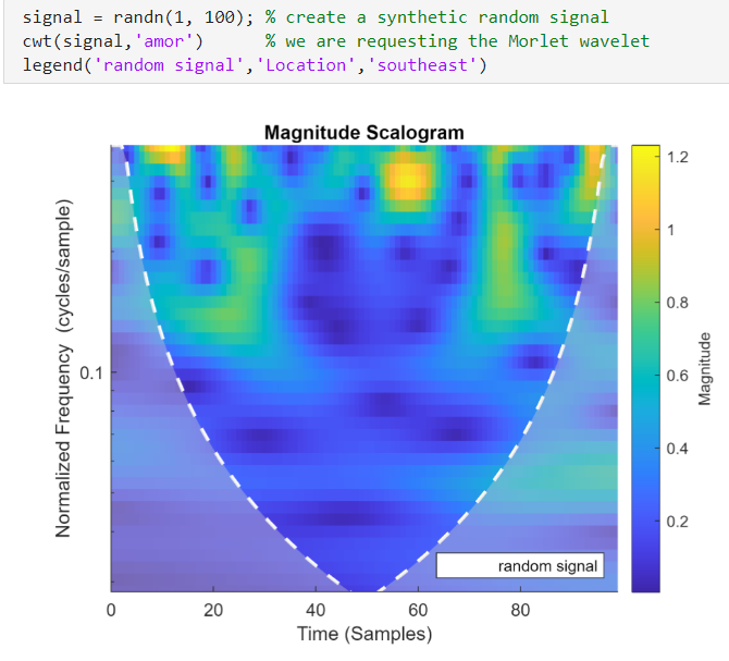
Matlab cwt function
The Matlab function cwt by default uses the Morlet wavelet. It performs the CWT on a given signal and returns several outputs.
The primary output of the cwt is the matrix of the wavelet coefficients
- each row is a scale (or frequency)
- each column is a position in time in the input signal These coefficients represent how closely the signal matches the wavelet at each scale and position.
- The value of each entry of the matrix reflects the amplitude (or energy) of the signal at particular frequency and time
The coefficients are complex numbers and they provide both magnitude and phase information (in real application is common to use consider only magnitude).
 The scales usually progress logarithmically from high frequencies (small scale factors) to low frequencies (large scale factors).
Each column represents a different time point in the signal. The granularity of these time points depends on the sampling rate of the original signal and the parameters of the wavelet. We remind that the normalized frequency is defined as
The cone of influence shows where the edges effects become significant is also plotted. The Gray regions outside the dashed white line delineate regions where edge effects are significant.
Inverse Continuos Wavelet Transform (ICWT)
The ICWT is the process of reconstructing a signal from its wavelet coefficients obtained through the CWT. The ICWT formula is:
is the matrix of the wavelet coefficients, where and are the scale and translation parameters. is the mother wavelet function is a constant specific to the wavelet used.
The meaning of the formula is that by integrating over all scales and translation, the contribution of all wavelets are summed to created the original signal.
The reconstruction accuracy depends from the choice of the mother wavelet
The time complexity is comparable to that of the CWT.