SC - Lezione 20 - Computing Derivatives Finite Differences

---

SC - Lezione 20 §

---

Checklist §

Domande, Keyword e Vocabulary §

• Computing Derivatives
• Finite Differences
• Taylor Series
• Forward Difference Formula
• Backward Difference Formula
• Central Difference Formula -
• Algorithmic derivation of general FD formulas
• Effect of the stepsize on FD
• Epsilon Machina
• Differentiation Matrix
• Toeplitz Matrices
• Diff. operator
• FD and polynomial interpretation
• FD for partial derivatives
• FD for the gradient
• FD for the Laplacian

Appunti SC - Lezione 20 §

Finite Difference formula §

A Finite Difference (FD) formula is an algebraic formula that approximates the value of the derivative (of a certain order) of a given function at a point. We can use either Taylor series or algebraic polynomial interpolation.

Taylor Series §

Infinite sums of derivatives at multiplied by the distance of the two points and ofcourse raised to power.

Forward difference formula §

It’s used for computing the first derivative. We simply stop at the first order of the Taylor Series.

From which we obtain the formula:

With an error of

Backward difference formula §

We simply start from the Taylor series expansion at (instead of x + h) and get the backward difference approximation:

With an error of

Central difference formula §

We combine the two previous difference formula to get a smaller error. More formaly we consider the Taylor series expansion of and up to the order around :

Then we do the following subtraction:

It’s more accurate than the backward/forward difference formula:

With an error of

Higher-Order Derivatives §

For example the second derivatives approximation by considering and and we can do:

By truncating the Taylor series to a desired level of accuracy and rearranging the terms, various FD formulas for first and higher-order derivatives are obtained.

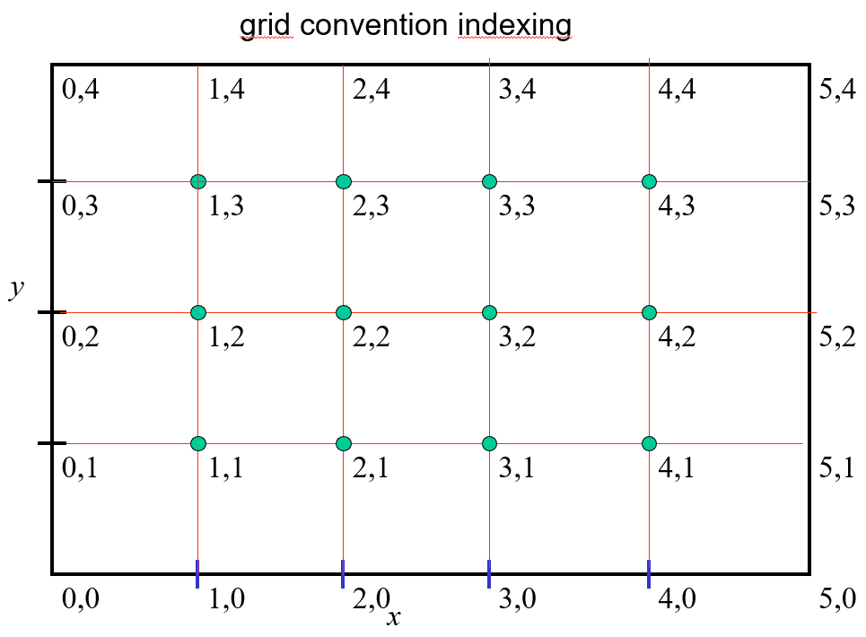
Derivative of a function on a grid §

In most applications we want to compute approximations of a derivative of a function on a grid.

A grid is a discrete set of points of

If i have a function of points, i want the derivative of points. In this context we have a grid (i.e a vector of points) and the correspondin values of the function (i.e a vector of values).

To approximate derivatives at these grid points, use Finite Difference formulas to compute: We want to approximate the derivatives of on the grid by means of . The latter values are obtained applying the FD formula.

in other words: To approximate derivatives at these grid points, use Finite Difference formulas to compute: …

Algorithmic derivation of general FD formulas §

I have a system of 5 equations in 5 unknowns. Where the unknonws are the derivatives: Notice how appears multiplied by each derivative of .

Then i write this system in matrix form as: is the coefficient matrix for example the first component on the first row of the matrix A, will be 1, the second will be -2, the third +2 , the fourth -4/3 and so on. (I coefficienti i numerini per cui moltiplichi d)

the solution of the linear system is

With this approach i can derive any formula of the derivative of any grade.

Effect of the stepsize on FD §

If i take the smallest possible, i have the maximum accuracy.

If i take the smallest possible, i have the maximum accuracy. In a digital context the optimal choice is where is the machine epsilon of floating point arithmetic.

where

We consider the minimum of the function , that is: ->

The optimal value is and the minimum error is

Note: Consider the function E:

• if is large, it is convenient to decrease it, since the term dominates.
• But, if is small, the term dominates and the approximate will worsten if you decrease

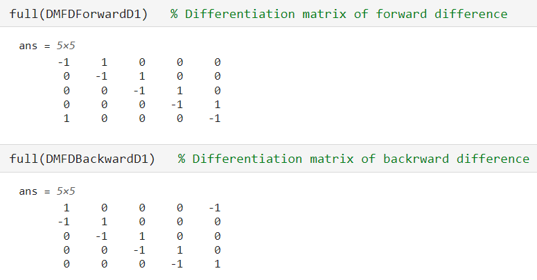
Differentiation Matrix §

FD formulas on a grid can be implemented as matrix-vector multiplication.

Since the differentiation is a continuos linear operator i.e

and the linearity property is retained by its discrete counterpart.

Each FD formula has an associated Differentiation matrix.

Toeplitz matrices §

All differentation matrices are toeplitz matrices that have the equal values on the diagonal

Differentation operator §

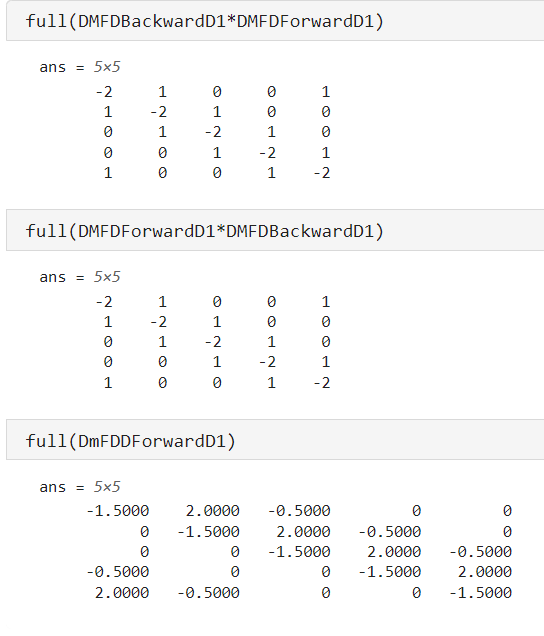
The Differentiation matrix for the central difference formula for the second derivative can be obtained as the product of two Differentiation matrices for first derivative, namely the differentiation matrix for forward difference times the differentiation matrix for backward difference.

In fact in calculus we define the second derivative as the first derivative of first derivative.

FD for partial derivatives §

FD can be extendend to functions of several variables and partial derivatives.

Let us consider a function and 2D grid ; with constant stepsize

and denote as the value

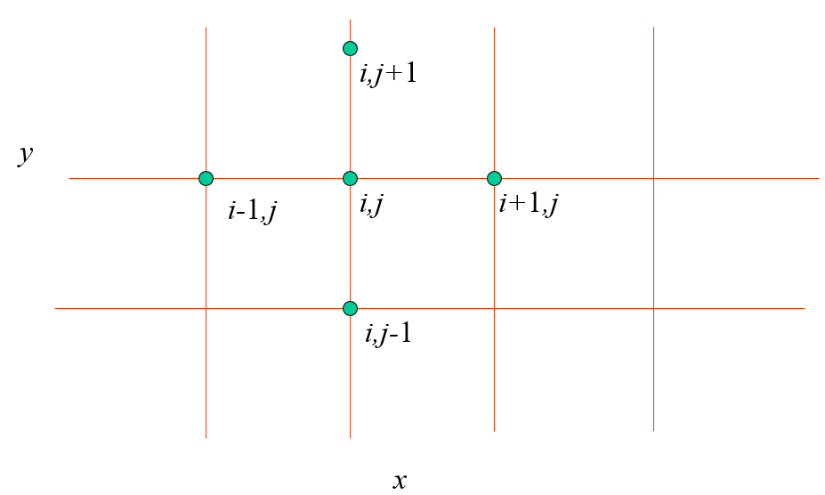
The forward difference formula, for the partial derivative rispect to x:

Another example, the central difference of the first derivative, partial derivative w.r.t :

FD for the gradient §

In Matlab you can use the ”gradient” function to compute the approximated value of . Matlab uses the central difference formula for computing the gradient inner a grid and forward/backward formula at left/right boundary.

Image example §

We consider an image and compute the gradient and we get two image one represent the partial derivative respect to x and the other respect to y

In the example we show that using the gradient Matlab function is more accurate rather than using the backward difference method that provides only a first-order accuracy.

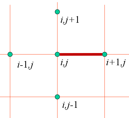
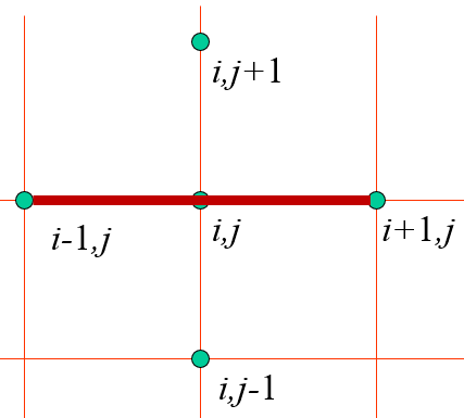
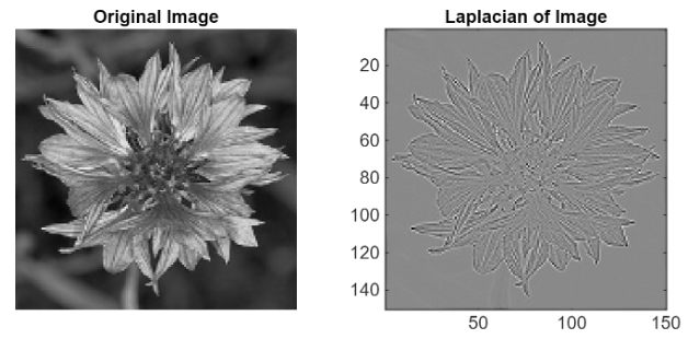
FD for the Laplacian §

Recall that the laplacian is the “trace” of the hessian matrix (the matrix of 2nd derivatives in multivariate functions. Trace means it’s the sum of all the derivatives in the hessian matrix. I.e we consider this laplacian:

We apply the central difference formula and get:

that gives this five-points stencil approximation of the Laplacian

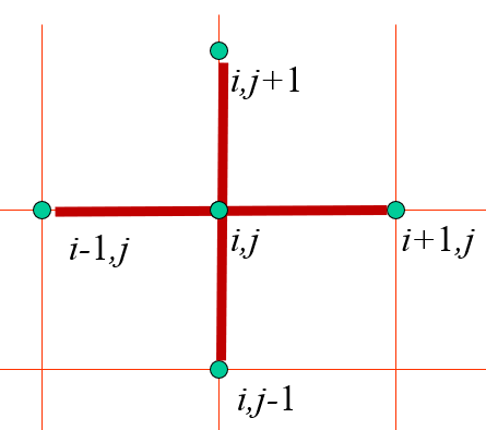
Since the derivative is a linear operator, notice that it’s exactly like doing first the derivative respect to , with the central fd formula and taking the same points on the grid from the previous example (see FD for partial derivatives), then do the same with derivative respect to and put the two together.

We see in an example that the laplacian can be used on image too, uses more informations (2 derivative of the function), so the edges are quite good represented, better than using the gradient.

---

Sommario §

Nota: In pratica ti devi ricordare le 3 difference formula, le immagini della griglia e delle linee rosse. E ricordare il fatto che la differenziazione su una griglia è un prodotto matrice vettore Basta sapere che esiste l’algoritmo per derivare le formule non c’è bisogno che lo impari a memoria.