DST Lezione 19
Sources:
- Fundamentals of Database Systems Seventh Edition | Chapter 24.4
- AWS DynamoDB Documentation
Key-Value Stores
The key-value is a primitive database form in which you identifty data with a key. All the data has this shape:
<k1,v>
<k2,v>
...
k, is the key, the unique identifier associated with the data item;vis the value that can be anything from a single number to a BLOB or a collaction of items.
Characteristics of a KV Store
NoSQL
- NOSQL means no sql as query language, no nested query, no optimization plan. What you get here you can retrieve it only by looking at the key;
Index Organized Table
- Most of the time the physical structure is an hash table and in more rare cases an heap file and a
-Tree, in particular an Index Organized Table (i.e. without auxiliary file);
GET operation
- The only query that you can do is restriction, here is called “get” and requires a key.
Schemaless
There is no schema, this has some implications. Say we have a collection of students
No JOIN operation
A key value store is joinless - we can have multiple table but we cannot have foreign key, everything is independent.
Choosing the key
Let’s talk about picking the right key for data. Say you’ve got student records. We could use something like the student matricola (ID) number as your key. So i will have a key value store with a structure like this:
But this id is meaningless for most queries. Say i want to search a students by last name with surname='ROSSI'. I have to do a full scan of the whole table and that’s heavy. For example, think of a nested query: that would require multiple full scan.
A solution could be a composed key with matricola and surname:
Now, if i want to query by name, i also have to do a full scan. If i recursively build composite index i will end up with a record of students with a composite key of all the fields. Basically what i have done is building a relational schema again. This is ofcourse not an optimal solution.
So, you gotta find a sweet spot—somewhere between a meaningless auto-incrementing key and a full-on schema rebuild. Think about how you’ll be searching your data, and build your key accordingly. If you’re often looking up students by department, toss department info into your key, and so on.
Fingerprinting
When it comes to building the key value system, a cool strategy for choosing the key is called fingerprinting; instead of copying the whole record you build a new artificial field based on values in a predictible way. Take the Italian Codice Fiscale, for example—it’s one string that packs in details like surname, name, birth date, and the city code where Mario was born.
Let’s say i wanna search by surname, using Codice Fiscale as my key, i’ve got all the info right there. In any case i have to full scan only the index, but it’s way cheaper than scanning the whole table.
Indexed fields
In real system there is a feature called indexed fields:
- use index and matricola as key
- add as indexed fields surname, name, region
Dynamo DB
DynamoDB is the default amazon product on AWS platform. A table in Dynamo DB does not have a schema; it holds a collection of self-describing items. It will uses JSON for data interchanging. In JSON data you don’t have a fixed structure.
Basic types are:
- Strings
- Numbers
- Document: is how JSON calls files
- Sets: set of numbers or string You don’t have any other primary type. If you want date for example you have to be creative like for example you could use the unix notation.
Physicial storage of dynamo db
- A table is called collection
- A record is called item
You “create tables” but these are not really tables: they’re collection. They’re not table but they have no schema. For the same reason an item isn’t a record.
When a table is created, it is required to specify a table name and a primary key. The latter will be used to rapidly locate the items in the table. The primary key can be either a single attribute used to build an hash index on the items in the table, or a pair of attributes. If you use a pair of attributes, the primary key will be a pair of attributes (A,B): attribute A is used for hashing, while B is used for ordering records with the same A value.
-
A is called partition key
-
B is called sorting key
-
https://aws.amazon.com/blogs/database/choosing-the-right-dynamodb-partition-key/
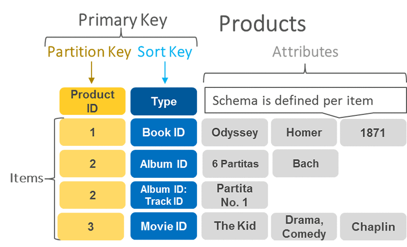
For example, in the notation we used:
[]=CS department
[]=Telecommunications department

in Cs department we put the matricola
[123
124
130
...
]
Since it is an hash, it costs me O(1) to find a record if i have the key. The second level (sorting key) is a sparse index so the cost will still be very low.
Consider the previous example. If i want to retrieve students by surname this doesn’t work and i should do a full scan. To avoid this i could build a secondary index by adding “surname” to the record. I build this in a separate file, so it’s called logical index. (recall the pointer is to the primary key, in this case to the department and matricola). I could also project other attributed if needed. In this way i don’t have to find the surname and then look to the data to read the surname, since i laready have it into the index.
Ofcourse, there is a strong limitation on how many secondary index you can build because: they are dense, they need a lot of space and they need computational power because they need to be updated. In DynamoDB there is a limit of 10GB for each partition, that scales automatically and you have atleast three copies of each partition.
When building these systems you cannot always reason “in advance”; the system must be build according to the most executed queries and other factors.
Consistent Hashing
It’s a technique used to manage scaling and different partitions. It reminds a bit the spiral hashing.
Say you have a list of servers (A,B,C) and each one may have different computational power: A=5, B=3, C=2. I need an hash function that applies to the keys of my items and gives me an angle. Each area between one point and the next, goes to the next (clockwise) server. For example in an area between A and C, where A < C, the output is assigned to C.
The advantage, like for spiral hashing is to avoid the complete reorganization of the data since only local reorganization is done in place. In this way, it’s more efficient to scal up & down the system.
Each partition on dynamo db have multiple copies on multiple server and AWS offer zone replication where you have replication of data in different geographically located data servers.
Strong and eventual consistency in DynamoDB
If you want strong consistency on Dynamo DB, then your throughtpute halves. This because the drowback slows down the system because of synchrnozation. The problem for eventual consistency is that you have three copies of the data that are not necessary coherent. If this is a problem or not, it depends on the application. For most application eventual consistency is enough because, aws data server synchronize in milliseconds.
The unit of memory is 4KB and you have two IO operations:
- WCU - Write Capacity Unit - default is 1000, divided by two for strong consistency
- RCU - Write Capacity Unit - default is 3000
Let’s take the example from Amazon DynamoDB documentation:
Say i want to read 80 items per second from a table. The size of these items is 3KB and you want strongly consistent reads. each read requires one provisioned read capacity unit. To determine this number, divide the item size of the operation by 4 KB. Then, round up to the nearest whole number, as shown in the following example:
- 3 KB / 4 KB = 0.75 or 1 read capacity unit
As we studied in previous lection, we have that
Dynamo DB Streams
Documentation say that:
Many applications benefit from capturing changes to items stored in a DynamoDB table, at the point in time when such changes occur. The following are some example use cases: DynamoDB supports streaming of item-level change data capture records in near-real time. You can build applications that consume these streams and take action based on the contents.
Buzzwords for saying it’s a log file.