HPC - Lecture 1-2
HPC - Lecture 1 - Introduction
- What is High Performance computing? Solve large-scale computational problem in “real time” (i.e. in useful time)
- Many modern applications require: processing very large datasets, producing results in real time and handling complex computational models
Von Neumann machine
- In 1945 John Von Neumann introduced an electronic computer scheme, based on the concept of “memorized program”
- The instructions are recorded in the “memory” in numerical form
- Input Unit, CPU, Memory, Output Unit,
- CPU: Control unit and Arithmetic logic unit
Big Data Problems
- Applications: weather forecasts, medical imaging, finacial data anlysis, cybersecurity, climate modelling, machine learning, big data analytics
- Big Data Analytics: elaborate large scale data
- many modern applications require: processing very large datasets, producing results in real time (or just in time!) and handling complex computational models
- just in time: in tempo utile
Software run time:
is a multiplicative constant which can depend on practical and stochastic factors: memory access, scheduling, etc. = execution tome of 1 floating point (f.p) operation, also called flops, s=seconds
How to reduce
- N. Trefethen quote “the fundamental law of computer science: as machines become more powerful, the efficiency of algorithms grows more important, not less”
- reducing
depends on technology (miniaturization process)
How to improve technology (history, skip)
- Almost 80 years ago, in 1945, the first computer was a supercomputer
- Von Neumann Machine, still basic scheme of nowdays computers
- 1946 ENIAC uses thermoionic valves
- Miniaturized transistors, first compute with integrated circurs ibm 360 in 1964
- 1965-1978 first commercial computer based on chip
- how many transistors can stay on a chip? MOORE forecast: transistors on a chip double.
- in 1975 Moore slightly changed his prediction: the computing power of micropro will double each 18 months
- this law has been reflected in practice ofr over 60 years and has established a virtuos cycle, pushing technological advances towards better, cheaper products.
- We have reached the technological limit, where we cannot get any better because we cannot miniaturize indefinitely
- Quantum computers are a very recent technology, that redefine the concept of memory. They replace traditional binary storage with unique quantum bits (qubits) enabling near-instantaneous data processing and retrieval. Quantum algorithms are designed to run on quantum computers. Despite the advantages obtained, these need important conceptual changes to standard algorithms.
Back to how to reduce
- reducing
has a tech limit - reducint
to optimize the algorithm also has a stop - Another way is parallel computing:
.
Parallel computing:
- parallel computing advances serial computing by simulating simultaneous complex events, similar to those in the natural world
- Parallel computing solves a problem by:
- dividing it into independent subproblems
- executing them simultaneously
- using multiple processing units
- Goal: reduce execution time by exploiting concurrency
Lecture 2 - Flynn Taxonomy
We have to solve “large scale” (or big data problems) in real time or useful time, so we need to increase software performance.
Temporal parallelism
Parallelism on chip: multiple functional units inside a single ALU (arithmetic logic unit) Temporal parallelism: many functional units that can be used for computing, in general operations are done step by step, each unit in the ALU can be used to execute a step (i.e 5 step in the slide) we can organize operation one after the other, such that at step 1 there will be only the first unit, at the step 2 there will be both 1 and 2, and then in 5 steps we will saturate the ALU, and from that moment on we will have 5 operations at the same time.
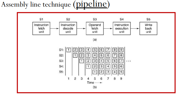
This is also called pipelining.
Pipelining Assuming that the different phases of the operation are separable, they are assigned to different functional units, so that when the first unit finishes its work for a phase, it can be dedicated to the next one
The use of pipelined functional units is also the basis of array processor capable to operate efficiently on data structured in array format.
The use of pipelined functional unit is also the basis of array processors: capable to operate efficiently on data structured in array format.
Flynn’s taxonomy
Michael J.Flynn beings to classify computers in:
- SISD or monoprocessor
- MISD: multiple instruction single data.
If we have also streaming of data, we have pipeline. But if we don’t put a stream, its not a piepline.
Pipeline critical issues
The first problem arises from the parallel work of units:
- Suppose the pipelined CPU needs to be execute the following code:
- These cannot be parallelized because the second must wait for the first one to finish
The second problem consists of conditioned jumps (IF this then …) If the code contains a conditional instruction (logical condition) and this condition is not met, the serial flux of code is interrupted and shifts to a different part of teh code.
Whenever this happens, the microprocessor must perform different operations, then empty the pipeline to upload the new data.
Obviously, these operations delay the execution.
Spatial Parallelism - Second type of parallelism (multiple ALU)
To overcome these intrinsic limits of temporal parallelism, a higher level of parallelism involving several processors synchronously or asynchronously was introduced.
The easiest solution is to implement is put several ALU. A single control unit manages multiple ALU, so the instruction is one but can be executed on multiple ALU. We can compute an array at the same time with all the data. There isn’t anymore that delay because we operate on every at the same time.
This kind of calculator, in the Fynn classification is a SIMD: Single Instruction Multiple Data.
Spatial Parallelism Synchronous
- Several arithmetic-logic units (ALU) operate following a single control (CU) running in parallel the same instruction on different data
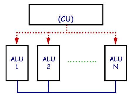
- The Cray-1 (1976) was the first one
- SIMD (Array Processors, connection machine 1988)
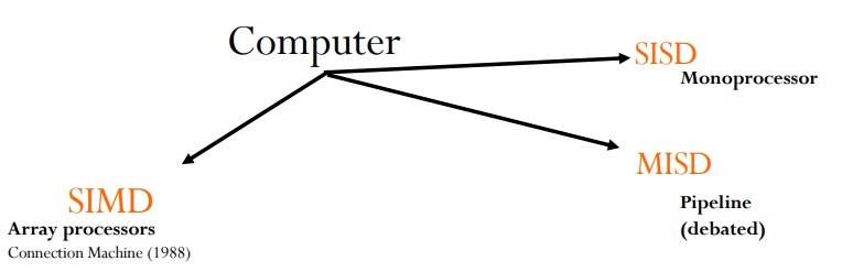
With more ALU, a single flow of instructions operates simultaneously across all units. This increases the number of instructions processed per second, although it does not eliminate operand upload latency. Remember this observation when we will talk about GPU.
Third type of parallelism: asynchronous
We have different processors cooperate by executing different instructions on different data. Parallelism involving several CPU=ALU + CU
This is called MIMD: multiple instruction multiple data, we have more computing unit for each ALUs.
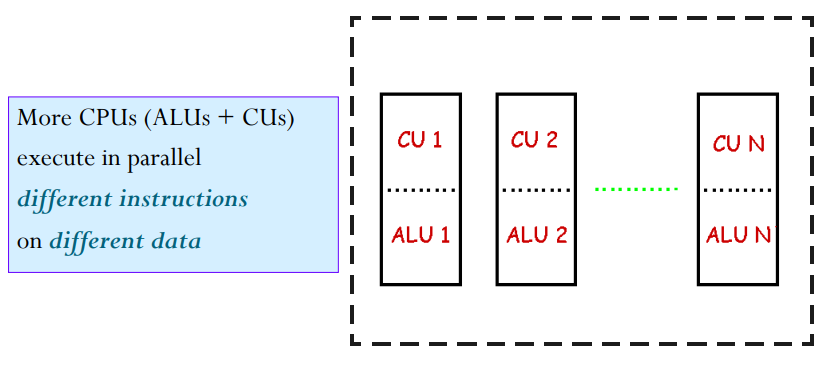
Technically this can be implemented in various ways, leading to various subcategories
MIMD-DM and MIMD-SM
MIMD (Multiple Instruction Multiple Data) represents asynchronous parallelism, where multiple processors cooperate by executing different instructions on distinct data sets. In this paradigm, each computing unit consists of a full CPU (ALU + CU). The implementation of MIMD is primarily distinguished by its memory architecture.
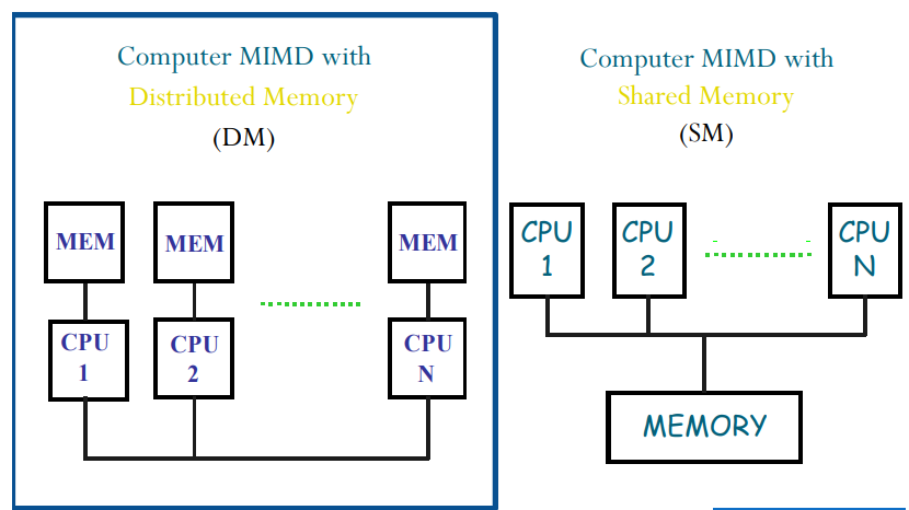
MIMD-DM (Distributed Memory)
In the MIMD-DM model, each CPU is paired with its own private memory. While the processors are interconnected to coordinate tasks, the memory used for processing the problem is physically distributed.
- Massive Parallel Processors (MPP): High-end systems such as the IBM RS/6000 SP, which utilized RISC (Reduced Instruction Set Computing) and a star topology linked via a proprietary IBM switch. Other notable architectures include the Intel TeraFLOPS.
- Clusters: A cost-effective alternative to proprietary MPPs. Clusters are sets of autonomous computers connected through standard I/O interconnects and network cabling, rather than specialized internal switches.
MIMD-DSM (Distributed Shared Memory)
MIMD-DSM architectures utilize virtual shared memory to provide a unified memory abstraction over physically distributed hardware.
- Example: The Cray T3E.
- Modern Implementations: Top-tier supercomputers (ref. top500.org) like El Capitan are essentially MPPs built with a cluster-like structure. They consist of numerous “blades” connected via high-bandwidth networks like the HPE Slingshot (12.8 Tb/s), utilizing sophisticated topologies to minimize latency between distributed nodes.
MIMD-SM (Shared Memory)
The first one is the Symmetric Multi Processor (SMP) used to indicate a multiprocessor architecture in which there are two or more identical processors connected to a single shared memory. The most prominent example is the modern multi-core computer.
This design introduces a second type of on-chip parallelism:
- First Type (ILP): Instruction Level Parallelism utilizing multiple ALUs and pipelining.
- Second Type (TLP): Thread Level Parallelism, where each core performs independent operations.
Shared Memory (SM) vs. Distributed Memory (DM):
- In SM systems, all cores share the same memory, making the distribution of subproblems across threads more efficient than assigning separate processes. However, these systems face a significant bottleneck at the system bus during concurrent memory access.
Does Moore’s law still hold true?
- It is clear that to ensure that the prediction is still valid we undoubtedly need parallelism
Right now intel is trying to do 3D chips, but right now there are GPU that are more efficient.
Currently all processors are parallel, they use different forms of parallelism and no system can be defined purely sequential anymore.
When we studied Distributed and parallel computing we saw the formula
On server there are something like 256 cores, while on laptop no more than 10-12, so it largely depend on the hardware.
Revisiting of Moore’s Law
“The processor is the new transistor” (Rowen): now it’s the number of cores per chip that double every two years.
Almost true (for server chips) but: we have Amdahl’s Law! (and a bottleneck to the memory). We can zero the parallel part but the sequential part has always the same. There is an issue in considering the “increasing” of number of cores per chip ofcourse because memory is still a bottleneck.
Possible hardware configurations
- Intel make all identical cores
- IBM/Sony/Toshiba cell: core of different size and function i.e specialized cores or grouped into SIMD units.
- Sun Niagara: only small and equal cores specialized
- Many small core and different: like NVIDIA GPU, many small cure but different, it is also called “many core”
Previous ones are example of Asymmetric Multi Processor
Example of asymmetric is the playstation 5: 1 GPU and 8 CPUs.
Graphics Processing Units (GPU)
There are three primary categories of GPU architectures, each optimized for specific workloads:
- Quadro (Professional/Graphics): Tailored for high-end graphics modeling.
- RDNA 2 (Gaming): Designed for consumer-level gaming performance.
- Tesla (Compute): Specialized for high-performance computing (HPC) where data integrity is critical; every data point is read and written with strict error control.
Key Architectural Differences
- Memory Capacity: Gaming cards typically feature less memory, as real-time rendering for games is less memory-intensive than complex mathematical modeling.
- Cooling Mechanisms: Gaming GPUs are engineered to operate quieter, whereas professional graphics cards are often noisier due to different thermal requirements.
- Drivers and Accuracy:
- Professional Graphics cards focus on 100% accuracy. They perform double precision calculations at full speed to ensure perfectly rendered images and mathematical rigour.
- Gaming cards prioritize throughput and speed. Their drivers may utilize rendering tricks to decrease accuracy in ways that are imperceptible to the human eye during high-speed frame transitions (e.g., high frame rates), ensuring smoother gameplay.
Evolution and Course Scope
The GPU architecture has undergone rapid evolution, effectively integrating nearly all established forms of parallelism. This course focuses on:
- GPU-parallel architectures: Understanding the underlying hardware structure.
- Tools and Algorithms: Developing the necessary framework to solve computational problems using these many-core systems.