HPC - Lecture 3 - Thinking in Parallel
The problem-solving chain of a parallel problem is the following:
- Consider a problem P
- Design a mathematical model M(P)
- Then convert this into a numerical model
- From this numerical model you can develop an algorithm
and/or a software
Recall that the fundamental formula that measures the execution time of serial software is:
We want to reduce
can be reduced optimizing the algorithm, however at some point we created algorithms so optimized that we don’t know how to futher improve can be reducing by improving the technology, but at some point we reach a plateau
The solution is parallel computing:
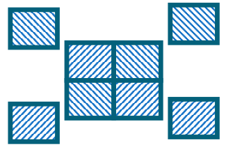
Parallel computing decompose a problem in multiple subproblems and solve them simultaneously using multiple processing units:
This creates a new perspective on the problem-solving chain:
- A parallel numerical model
is created - Then a parallel algorithm and a parallel software are created
and .
Discretized Method: consider a discretized method where the steps are organized in
Functional Decomposition
One option is functional decomposition where each processing unit performs a different step.
Consider the discretized method, organized in steps
Characteristics:
- Scaling depends on the number of independent tasks
- Helpful only for sufficiently complex elaborations
- Applicable for a procedure charaterized by multiple computational basic cores.
Domain Decomposition
In domain decomposition all processing units perfom the same operation on a different subset of data.
Consider the discretized method, organized into steps
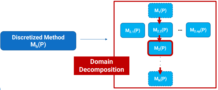
In domain decomposition we partition the data and process each subset uniformly.
Characteristics:
- Scalabe with the number of data elements
- Helpful only when there is a simple collection of local results
- Applicable for procedures with several consecutive computational kernels
A combination of the two previous approaches is also possible.
How to parallelize a numerical method
The first step consists in identify the fundamental computational kernels. Whatever the problem to be solved the basic computational kernels to parallelize are based on only two kinds of data structures: vectors and matrices.
Can you do parallelism on graphs and trees?
Yes, it is possible. Parallelism on vectors and matrices is often called regular parallelism because you know exactly where in memory i.e
matrix[i][j]are and hardware is optimized for operations on this kind of data structures. A new major research area in parallel computing is parallelism on irregular data structures like graphs and trees, where things get a little bit more complicated and it is out of scope of this note to explain that.
The second step consists in domain decomposition. To decompose the problem and solve it in parallel it is necessary to understand the concept of domain decomposition.
Computational Kernesl: Domain decomposition
Consider the problem of: computing the sum of N numbers:
On a single-processor computer, the sum is computed by performing N-1 additions e.g:
begin
	sumtot := a[0]
	for i=1 to N-1 do
		sumtot := sumtot + a[i]
	endfor
end
Decomposing this problems means decomposing the problem of size
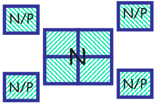
Divide the sum into partial sums and assign each partial sum to a processor/core. And then the partial sums must be combined properly to obtain the total sum.
Sum problem for MIMD-SM
Consider the MIMD Shared Memory architecture, and the sum operation. Example N=16, p=4.
Data must be distributed among processors:
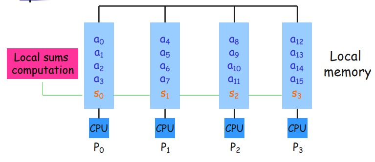
There are 3 strategies:
- Strategy I: each processor computes its own partial sum. At each step, each processor sends this value to a single predetermined processor. That processor contains the total sum.
- Strategy II: each processor computes its own partial sum. At each step, different pairs of processors communicate simultaneously. Then in each pair, one processor sends its partial sum to the other, which updates the result. The total sum is stored in a single predetermined processor.
- Streategy III: at each step:
- different pairs of processors communicate simultaneously
- in each pair the processors exchange their partial sums
- The total sum is stored on all processors.
The key feature required to implement these strategy is a way to make possible communication between processors. A software tool fo developing algorithms in a MIMD-DM computing environment is the Message Passing Interface (MPI).
Sum problem for MIMD-DM - Multicore
Now let’s consider the MIMD-DM environment. Cores can simultaneously access global memory on different data:
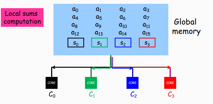
In order to update the value of the sumtot variable correctly, each core must have exclusive access to this variable during the last phase. Do this we need synchronization of memory access.
We have the following strategies:
- Strategy I: each core computes its own partial sum. Each core adds its own partial sum to a single predetermined value. The global sum is stored in the shared memory.
- Strategy II: each core computes its own partial sum. Half of cores (with respect to the previous step) compute a contribution to the partial sum. The global sum is stored in the shared memory.
- In this strategy both the partial sum and the contribution are concurrent operations
There is no third strategy since the result is always stored in the shared memory.
There are several tools for software development in MIMD-SM computing enviornment: OpenMP, Pthreads, Windows threads…
Problem: Matrix-Vector product
The problem is the design of a parallel algorithm to compute the product of a matrix
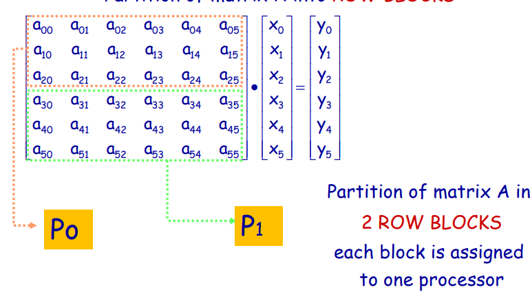
General idea: decompose a problem of size N into P subproblems of size N/P and solve them simultaneously on multiple processors. This can be done by partitioning the matrix into subblocks, that are distributed to the processing units.
We have the following strategies:
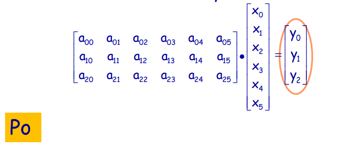
Strategy I: We partition a matrix
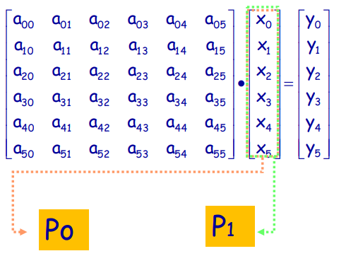
Strategy II: consists into partitioning a matrix
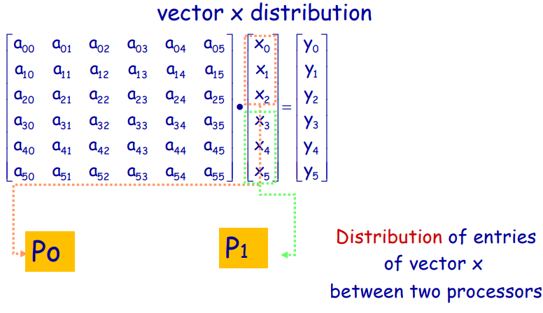
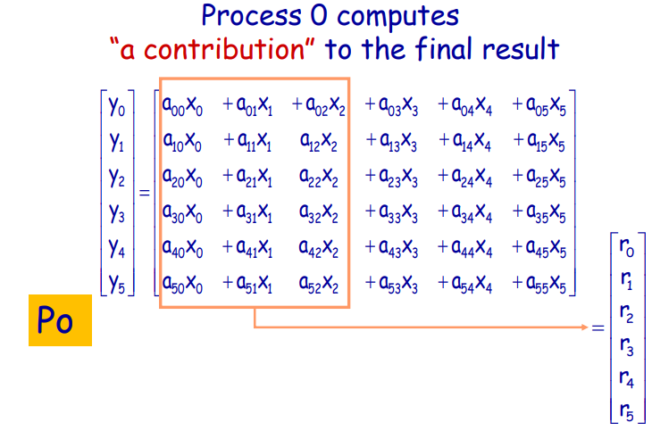 And so does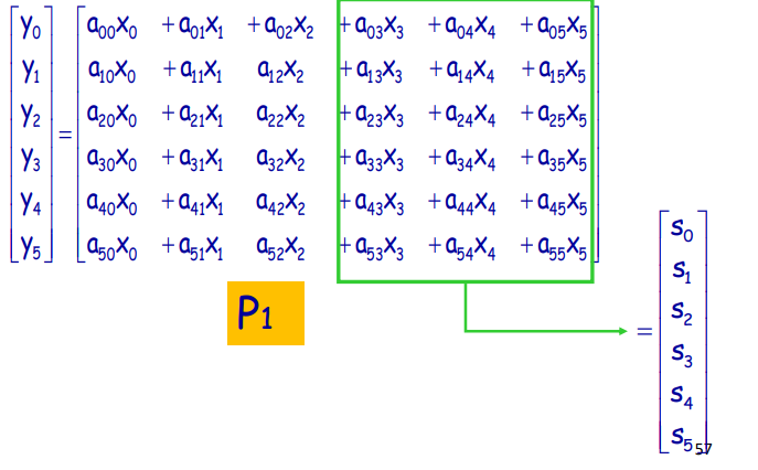
To obtain the final vector
Strategy III: it’s a combination of the previous two ones strategy: if we take row blocks and column blocks together we will have square blocks:
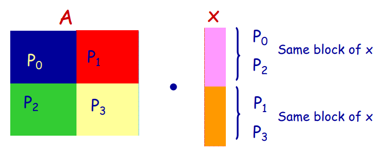
Each computes the following parts:
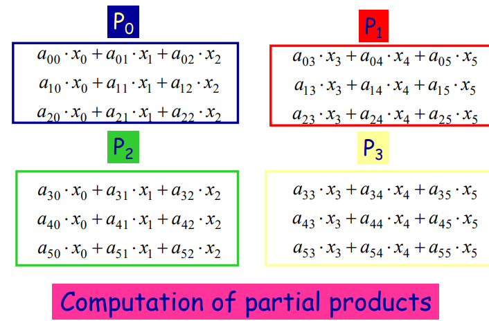
Then the partial products are first added together e.g. the result of 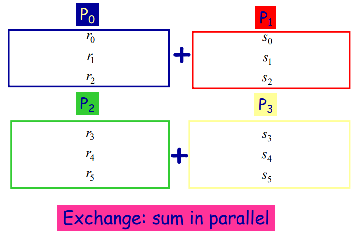 The processors must sum the partial results and exchange entries in order to compute the final result
Processors Grid
MPI provides APIs for defining the processor grid
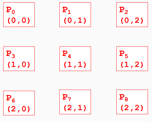
Matrix-Vector product for MIMD-SM
Consider a always
Strategy I: like before we have a subdivision of work on the matrix
Strategy II: We divide the matrix
Strategy III: the distribution of work on matrix
Efficiency of a parallel algorithm
Speed-up: measures the reduction, in terms of execution time, with respect to the sequential version of the algorithm:
The ideal speedup is
with total overhead:
it measures how much the speed-up differs from the ideal case.
Efficiency: measures how effectively the algorithm exploits the available parallelism:
Ideally: