SC - Lezione 24 - DFT, Complex Vector Space, Matrix Vector multiplication, IDFT, FFT algorithm
Checklist
Domande, Keyword e Vocabulary
- Scalar product, orthogonality and basis in complex vector space
- Geometric interpretation of the DFT matrix-vector multiplication
- Projecting from real space into complex space
- Exercise: DFT of the standard base vector of R
- Inverse DFT (synthesis)
- Does the inverse of the matrix
exists? - FFT algorithm
Appunti SC - Lezione 24
For complex matrices, symmetry is defined differently and is referred to as Hermitianity. The conjugate transpose (or Hermitian transpose) of a complex matrix
To compute
For real matrices, if 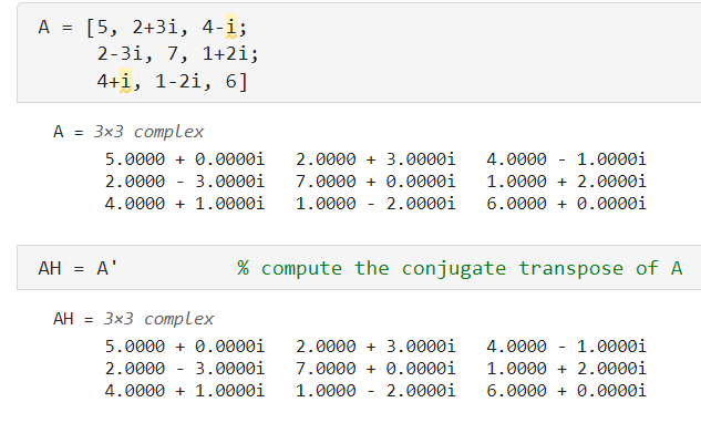
The matrix
Conjugate symmetry property:
where the bar denotes the complex conjugation.
When we have computed and shown the amplitude spectrum of a signal we display only the positive ones, one half of the spectrum. The reason is given by this “symmetry” of the matrix
From the “real part of the DFT matrix of order 256” image, we observed symmetry due to the cosine function, which is inherently symmetric.
In contrast, the phase DFT matrix of order 256 does not exhibit symmetry because it is based on the sine function, which increases in frequency and is not symmetric.
Scalar product, orthogonality and basis in complex vector spaces
One of the two vector must be a column vector.
In the case of complex numbers, there is no commutativity property because:
Which is different from
Two complex vectors
Nothing changes for the 2-norm definiton
The projection of a vector
It is worth nothing that if one of the two vectors is a real vector, then the complex scalar product becomes the standard scalar product.
Geometric Interpretation of the DFT
When you multiply the DFT matrix by a vector, it can be interpreted as a sequence of standard scalar products between the first row and the column. This means that you are projecting this vector onto the row.
The interpretation for the DFT is that you project your vector from the real space of dimension
Consider two distints rows of
When you multiply the DFT matrix by a vector, it can be interpreted as a sequence of standard scalar products between the first row and the column. This means that you are projecting this vector onto the complex space using the DFT matrix
Exercise: DFT of the standard base vectors of R^N
What happens when you apply the DFT to the identity matrix
At the middle point, you observe the highest frequency. Here, the sine and cosine components are identical, resulting in the maximum frequency. The cosine exhibits the maximum possible oscillations that can be represented on this grid. This middle index is referred to as the Nyquist Point.
Nyquist point
Inverse DFT
Also called synthesis, reconstruct the original time domain from its frequency domain. It’s the inverse operation of the DFT, called Inverse Discrete Fourier Transform
The only things that changes are:
- we don’t have the
sign in the exponent of (recall that it represents a complex number that is the root of unity) - We have to multiply by
(normalization)
We can also write this formula using the root of unity definition:
Here in the IDFT formula we have an exponential with positive exponent in contrast with the exponent of the DFT formula that is negative, as we defined it as root of unity with the minus sign:
Inverse of the DFT matrix
Even the IDFT is a matrix vector multiplication. First thing is to ask if does it exists an inverse? Yes because
The inverse of the matrix
And ofcourse each entry of this matrix is complex number
FFT algorithm
Key Idea of the FFT
The key idea is that we can apply a recursive algorithm, with a complexity of
Look at this fact:
If i have the root of unity and
Squaring
Dividing the signal into two DFTs
To compute the DFT of a vector of length 𝑁 by dividing it into two DFTs of length
We separate the even-indexed and odd-indexed elements, splitting the sum into two parts of length
- The even-indexed elements are represented as
; - The odd-indexed elements are represented as
; We recall this fact for explaining why we wrote and in the formula above.
Let
Then, we have that:
for
In order to get the second half of
Using the property that:
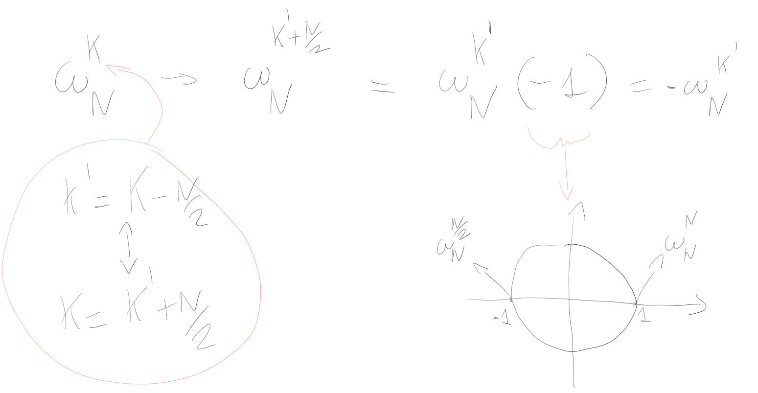
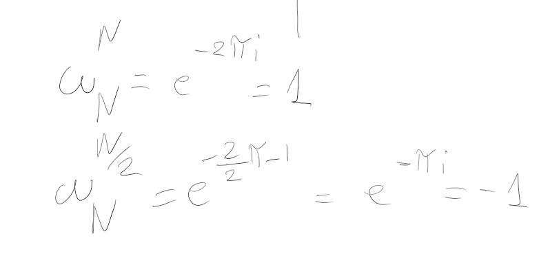
we find that the second half of
for
Formally:
for
The concatenation of the first part and second part of gives the final result
means concatenation of the left vector with the right vector
In summary, the FFT algorithm divides the DFT into smaller DFTs of sizes, typically powers of 2, using the well known Divide-and-Conquer approach. This is done recursively until reaching the base case of the DFT of size 1.
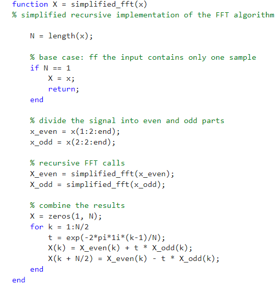
Special factorization of the DFT matrix
This idea of splitting the indexes, can be seen as particular factorization of the matrix
Suppose that we start with a
Where
We consider also this:
Then
If
An example of analysis and synthesis of audio signals
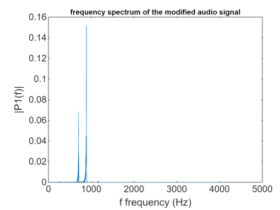
We have this situation in the frequency domain:
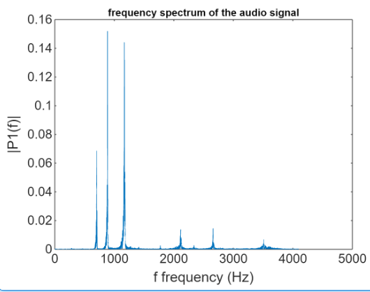 We then apply a modification of the signal:
X_modified(f > 900) = X_modified(f > 900) / 100;
it means that the frequencies higher than 900 are “smorzate” and the sound should be changes such that you hear less the higher frequencies.