SC - Lezione 4 - Projection Matrix, Recall of applications of scientific computing, Variance and Average, Product of block matrices, Orthogonal matrices, square matrices, matrix norm, rotation matrix

---

SC - Lezione 4

Domande, Keyword e Vocabulary

• Projection Matrix
• Least Square Fitting
• Product of block matrices
• Square Matrix
• Linear Transformation
• 2-norm = 1
• Mutually orthogonality
• Inverse Matrix of orthogonal matrix
• Rotation Matrix

Appunti SC - Lezione 4

Projection Matrix

In the formula we have:

• at the denominator we have a scalar product
• at the numerator we have an outer product So to simplify things we are dividing a matrix by a number. This particular matrix is called projection matrix.

Recall of elementary applications of Scientific Computing in Matlab

In the Matlab file the first two applications uses the Least Squares Fitting.

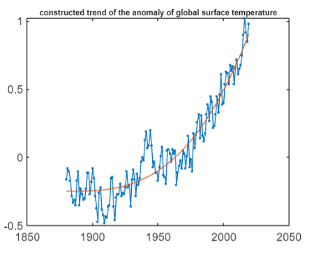
In the first application, i have the temperature in a period of time, but i consider just a subset of the time. I calculate the anomaly as the difference between the temperature and the average value.

Variance and Average

The average is the most representetive point, then you have another information that tells you how far the data is from this point, that is the variance. Data that is very close has a small variance, while the interval is very large.

If you have two large dataset, one with small variance and the other one with large variance, which one will have more information?

The larger the variance the more is the information. If we have data that is close to the average we have small informations.

Back to the application, i use the least square fitting with a third degree polynomial.

t_scal =(t-1880)/10;   % scaling and representation in decades
% plotting grid
tt = linspace(1880,2019,300);
tt_scal = (tt-1880)/10;
degreepol = 3;    % least squares with cubic polynomial
coef = polyfit(t_scal,at,degreepol);
pol = @(x) polyval(coef,(x-1880)/10);
figure;
plot(t,at,'.-')
hold on
fplot(pol,[1880 2019]); title('constructed trend of the anomaly of global surface temperature', FontSize=7)
set(gcf, 'Position', [100, 100, 400, 300]); % modify the size of the figurehold off 

First we represented the t_scal in lesser scale number and divide by 10 so it’s like working by decading instead of years. Linspace is used to create a grid. The polyfit function solves the Least Square Fitting problem. If i have the coefficients of the polynomial, i can use polyval to evaluate in any points the polynomial. @(x)is an anomymous function, and it is polyval of the coefficients in the interval i want.

Application 3 - product of block matrices

I have two matrices. A matrix and a matrx B and i want to compute C as matrix-matrix product.

Suppose that

We can partition the two matrices: and

Looking at the matrix i imagine that the matrix is composed of two submatrix. The first block is of size columns and the second one is of size . columns. has () columns. So, is an matrix. Now i perform the following partition on the following B: is a square block because i choose rows and , while has columns but rows. Notice we obtain two matrices so we can sum without problem the two to get C.

The computational complexity is the same either doing this or doing directly A*B

The quickest way to check if they are equal is to consider the difference of the two matrices, and then take the norm norm(C-A*B)

This result is ok, a better one would be obtained by doing norm(C-A*B)/norm(C) (or divided by the norm of the other matrix).

The interesting fact is, suppose your matrix has null blocks, null submatrix. Like an image with a white piece. The null block is null. Since is a zero block so multiplied by a matrix you get a zero matrix. So the matrix C is just equal to .

Remember this fact because we will use this in the next lesson.

Orthogonal Matrices and QR Factorization

Unitary Matrix and Orthogonal matrix are terms used to define the same thing. Usually unitary matrices are the ones with complex number. In this course we will refer to such matrices ad orthogonal.

A Square matrix Q is orthogonal if its columns have 2-norm = 1 and they are mutually orthogonal; This property can be described by the following property:

Also, an orthogonal matrix has orthonormal rows, that is:

Another important property that follows from the previous ones is that:

Per capire la proprietà si può considerare la prima interpretazione (vedi sul quaderno).

To understand why 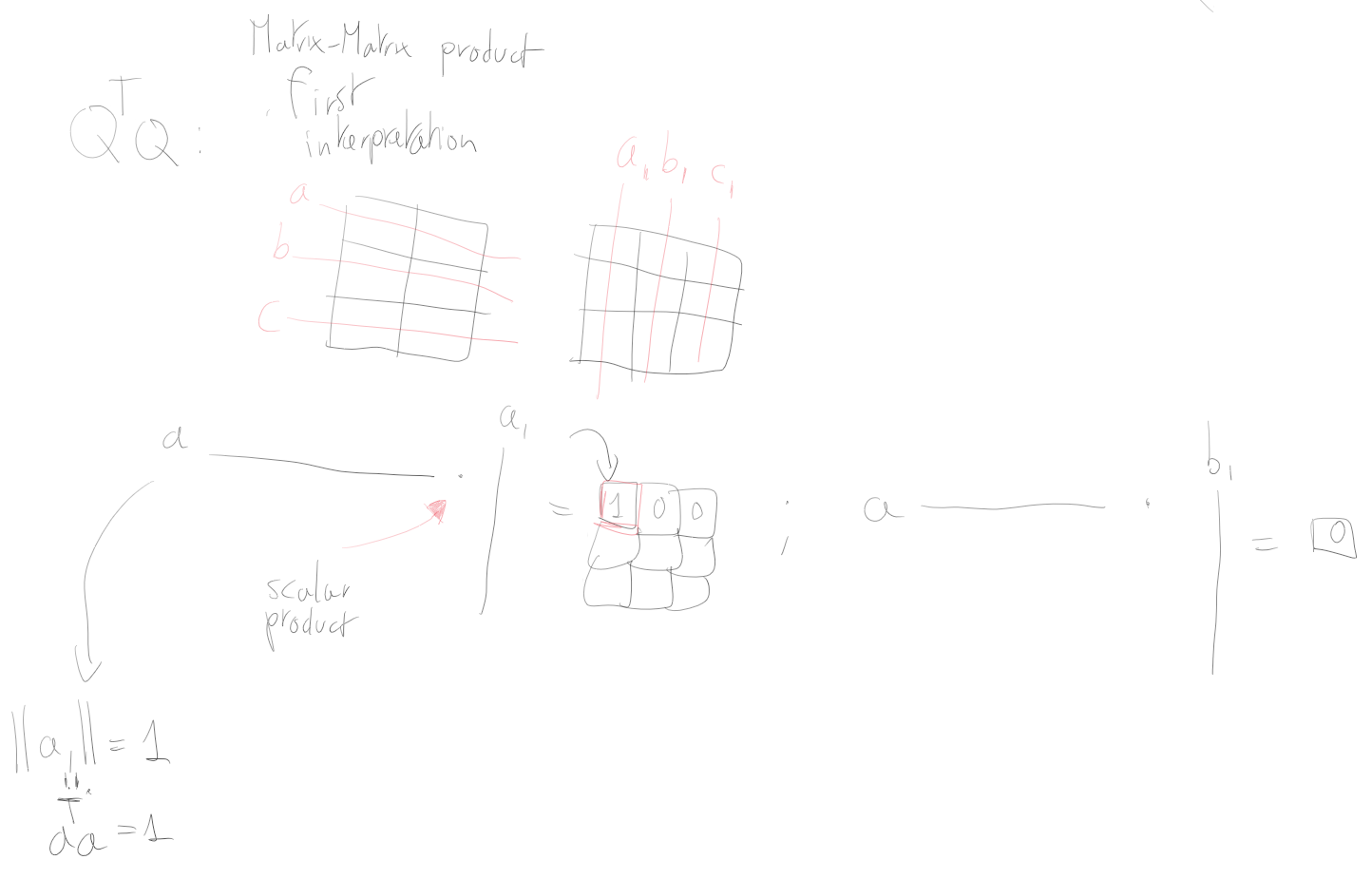see the matrix-matrix multiplication, first interpretation.

Inverse of a square matrix

Given a square matrix , if there exists a matrix such that , where is the identity matrix, is called the inverse of .

For these matrices, the inverse is the identity matrix, and it is straightforward to compute because it is obtained simply by taking the transpose.

Norm of an orthogonal matrix and implications

The 2-norm of an orthogonal matrix is always 1

If you have a vector, and you multiply this vector by a matrix you are doing a linear transformation of the vector. The 2-norm of a matrix tell us how much a vector is enlarged when multiplied by a matrix. What happens if the 2-norm is 1? Then the length remains the same.

The implication of this property is that these kind of matrices are rotation matrices, since only the direction of a vector changes when multiplied by this.

For example if Q is orthogonal and , then The norm remains unchanged when multiplied by the norm of an orthogonal matrix.

Example: Rotation of Yodapose

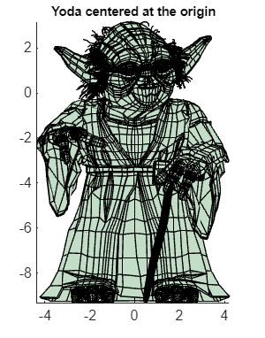Yodapose is a matrix that represents the 3D Yoga image. The image is composed of triangles, so to rotate them we need to first compute the centroid, then translate the centered origin of yoda in

centroid = mean(V); 
V0 = V-ones(size(V,1),1)*centroid;

The row of this matrix represents the vertices of the tridimensional vector that i want to rotate.

In this case it’s useful to consider the second interpretation of the matrix-vector.

To rotate triangles (See example of yodapose_low) we need to first compute the centroid, then traslate the centered origin of yoda in V0. Then, since the vertices of the vector tridismensional are the row of the matrix i want to apply to each row the transformation.

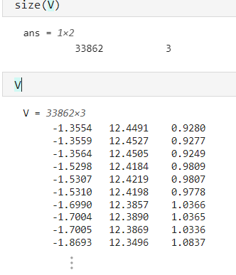V is the matrix that contains the vertices of the triangularization of the 3D Yoda.

I apply the second interpretation of matrix-vector, i have to transpose the vertices of the triangle.

I do the following operation: , where is first translated then multiplied. By using the second interpretation, the first column of the output is the first column of multiplied by Q and so on.

Consider as a collection of 33862 column vectors, each with 3 entries. When you multiply by , act on each column independently. It’s like doing a matrix-vector multiplication of and a vector of size . This is the Second interpretation of the matrix-matrix product, considering the result a matrix-vector product. Each column of the output matrix, is the matrix-vector product of the first matrix () by the j-th column of the second matrix .

If we don’t wanna transpose the vector for any reason, we can just transpose , see Transposition of matrix-vector equation of the previous lesson.

---