Bayesian Theory of Decision

Bayesan Theory of Decision §

See also:

• [[../../Statistics & Probability & Game Theory/Statistics/Probability, Sample Spaces and Events, Independent Event, Conditional Probability and Bayes Theorem (Statistics)|[STATISTICS] Probability, Sample Spaces and Events, Independent Event, Conditional Probability and Bayes Theorem]] for the statistics foundations required to understand this chapter
• Source: F.Camastra,A.Vinciarelli, Machine Learning for Audio, Image and Video Analysis, (5° Chapter)

The fundamental idea in BTD is that a decision problem can be solved using probabilistic considerations.

Dataset definition: consider a set of pairs that we call dataset.

Assume we have a dataset of i.i.d data: independent and identically distributed. This means they are drawn independently accordingly to the probability density .

Assume a binary classificator with two classes.

Assume all the relevant probabilities are known.

Bayes Theorem §

The Bayesian Decision Theory is based on this theorem: defined as:

• Reads as: the conditional probability of given datapoint is given by the conditional probability of given class multiplied by probability of class , normalized by the probability of

In the context of Bayes Theorem:

• : is called posterior probability
• is called likelihood
• is called prior probability
• is called evidence

Informally we say that:

Posterior Probability simplified formula §

Evidence in the case of two classes is calculated as:

Being a normalization factor, it can be neglected, and we can conclude that:

When is large, it is likely that sample belong to class .

Demonstration of the theorem §

Recall the definition of conditional probability (also called joint probability). The joint probability density of finding a pattern X in the class is:

But the same joint probability can also be written as:

Plugging equation the two equation together we have:

Divide by

Bayesian Decision Rule §

Intuition - Boys and Girls Example §

Imagine a classroom with boys and girls. The examiner has a list of surnames but doesn’t know each student’s gender. When a student comes forward after being called, they “reveal” which of the two possible states of nature they belong to.

States of Nature: the classroom is our natural world, the state of nature is the class label either a student is a boy or a girl .

Probabilistic assumption: since the examiner doesn’t know the true state (i.e if the student is a boy or girl) it make sense to treat as a random variable.

Prior Probability Decision Rule §

Before seeing anything else, the examiner only knows how many boys and girls are in the class. Let be the prior probability that the student is a boy, and the probability that the student is a girl.

With no extra information, the decision must rely on these priors:

Joint Probability Decision Rule §

We said that

When is large, it is likely that sample belong to class . We can theoretically demonstrate this.

Consider a binary classifier.

We observe that for a pattern , the probability of error is if we assign to . And viceversa. We can minimize by deciding if and , viceversa. We can compute the average probability of error as:

The probability error associated to Bayes decision rule is: .

Then, deciding if and otherwise, it is guaranteed that is as small as possible. Hence the following Bayes Decision Rule is justified:

If we plug the Bayes Theorem and neglect evidence we obtain that:

Optimality of Bayes Decision Rule: Bayes decision rule (or Bayes classifier) is optimal, i.e., no other rule (or classifier) exists that yields lower error.

Loss function §

In many academic papers, the concept of a “Loss Function” is frequently encountered.

When considering more than two classes we talk of a loss function. This lets the classifier take actions that aren’t simple class assignment for example, choosing to reject a decision.

postal OCR example

In postal OCR systems, the allowed error rate is extremely low. If the device reading an address makes more than 1.5% mistakes, the correct action is to reject the input rather than guess. A loss function makes this kind of behavior possible.

The loss function assigns a “cost” to every possible action. This cost turns classification errors into meaningful decisions, and lets us say that some mistakes are worse than others.

For instance, suppose that the cost of a misclassification of a pattern can depend by the apriori probability of the membership class. Misclassifying a pattern that belong to class can be considered heavier if is high.

Conditional and expected Risk §

• Let be the finite set of possible classes the pattern belong to
• Let be the set of the possible action of the classifier.
• Let be the posterior probability

The loss function measures the penalty we pay when the classifier takes action while the true class is .

Conditional risk is defined as:

• So for each possible true class, we multiply the penalty of choosing by the posterior probability of that class, and sum over all classes.

When we observe a pattern we choose the action that minimizes this conditional risk.

A decision rule is simply a function that outputs one action from the set for each input . For every the output is an element of the set .

Given a decision rule , the overall risk is:

In theory we want to minimize this, but in practice we can’t compute the integral because we only have a finite dataset.

So we replace it with the empirical risk:

• is the number of patterns in the dataset

This is essentially the Bayesian Decision Rule written in terms of the empirical risk. During training, the error we measure is the empirical risk.

As the dataset grows, the empirical risk approaches the expected risk, which is why we say that empirical risk is consistent:

Binary Classification Case §

We now apply the previous ideas to the special case of binary classification.

In this case, choosing means deciding that the pattern belongs to the class , and choosing means assigning it to class .

The conditional risks become:

The Baye decision rule becomes: Decide is otherwise decide

This same rule can also be expressed in terms of posterior probabilities.

To show this, we have to demonstrate that . Substituting the definitions:

Scambiando questi valori otteniamo:

And we obtain:

Since the posterior probabilities come from Bayes’ theorem, we substitute them explicitly (and drop the evidence term, which appears on both sides):

Now we isolate everything on one side:

• The right-hand side is called likelihood ratio
• The left-hand side acts as a threshold.

If the likelihood ratio exceeds this threshold—which does not depend on the particular pattern , then the decision is ; otherwise .

So the bayes decision rule in terms of posterior probabilities (binary case) becomes: Decide if Otherwise decide .

These expressions are positive because the loss associated with making an error for example is larger than the loss associated to a correct classification

We check this because if one of the terms were negative, the direction of the inequality would flip. In general, these quantities are positive.

In summary, the classifier compares the likelihood ratio:

with a threshold that does not depend on the pattern. If the ratio is larger, we choose otherwise .

Zero-One Loss Function §

In order to find a decision rule that minimizes the error rate, we must first degine an appropriate loss function.

The zero-one is a particular type of Loss function. Introducing a specific loss function is fundamental to do computations for the likelihood ratio disequation.

The zero-one loss fuction assigns 0 (correct) if the action is taken and the pattern belongs to , otherwise 1 (error).

Formally defined as:

• is the action that the classifier makes, is the class
• means the probability that the classifier take the action and the posterior probability is

Property: zero-one loss function assigns no penatly to the correct decision, and viceversa any error has penalty one. All errors are evaluated in the same way.

Now apply the zero-one loss function to the conditional risk, we get:

• is only for the correct case and for the remaining cases it’s .
• Therefore, we can rewrite the summation as because the only term that does not appear in this sum is when , i.e
• is always , a constant so it disappear from the summation
• Recall the the sum of the probabilities is one, therefore
  • to pass from left to right term, just add and subtract :
  • by definition (of probability) the first term plus is 1

We want to minimize , that corresponds to maximize . So when you use the minimization of the conditional risk that corresponds to pick the class with the highest posterior probability. It is the same principle of the bayes theorem: pick the class with the highest poerior probability.

Discriminant Functions §

The use of discriminant functions is a popular approach to make a classifier.

In neural networks, the output can be interpreted as a score, and classification is performed by comparing this score against thresholds. For example, if the output is larger than a certain threshold, the input is classified as belonging to Class A; otherwise, it belongs to Class B, and so on.

This approach can also be represented within the framework of Bayesian decision theory. By using discriminant functions, we temporarily set aside considerations of risk and conditional probabilities and adopt an alternative method. However, we will ultimately show that these two approaches are equivalent. Specifically, selecting the class with the highest discriminant function value is equivalent to selecting the class with the highest posterior probability.

Set of discriminant functions: Given a pattern , and the finite set of possible classess: we call: , with a set of discriminant functions.

Definition of discriminant function: with is a discriminant function.

Discriminant function rule §

Assign the pattern to the class if:

Assign the data point to the discriminant function whose output is the highest value for that datapoint.

Equivalence between discriminant function and bayesian rule §

Now we show that it is easy to represent a Bayes classifier in the framework of the discriminant functions.

For each conditional risk we define a discriminant function such that .

Consider the Zero-One Loss Function, ad apply the definition to get:

• we neglect as constant and obtain

Justification: An important property of discriminant functions is that they are not uniquely determined. If we add each function a constant, we get a new set of discriminant functions which produces the same classifications produced by the former set.

Now, using the explicit definition of posterior probability by Bayes Theorem, we obtain:

Let . We take the logarithm (log probability trick):

The evidence can be neglected hence we obtain as final formula:

Decision Regions: the use of such set of discriminant functions induces a partition a partition of , which is divided into decision regions, . If then . The decision regions are separated by boundaries that are hypersurfaces in .

Note

A surface has 3 dimensions, an hypersurface has more than 3 dimensions, i.e 4,5,100 dimensions

Discriminant Functions - Binary Classification Case §

In this case we have two classes, therefore two discriminant functions and .

The two can be combined in an unique discriminant function: .

A pattern is assigned to if and viceversa.

Decision Rule Binary Classification Discriminant Functions §

Decide if decide otherwise.

This is obivious because, is negative, when the second term is greater than the first, so when .

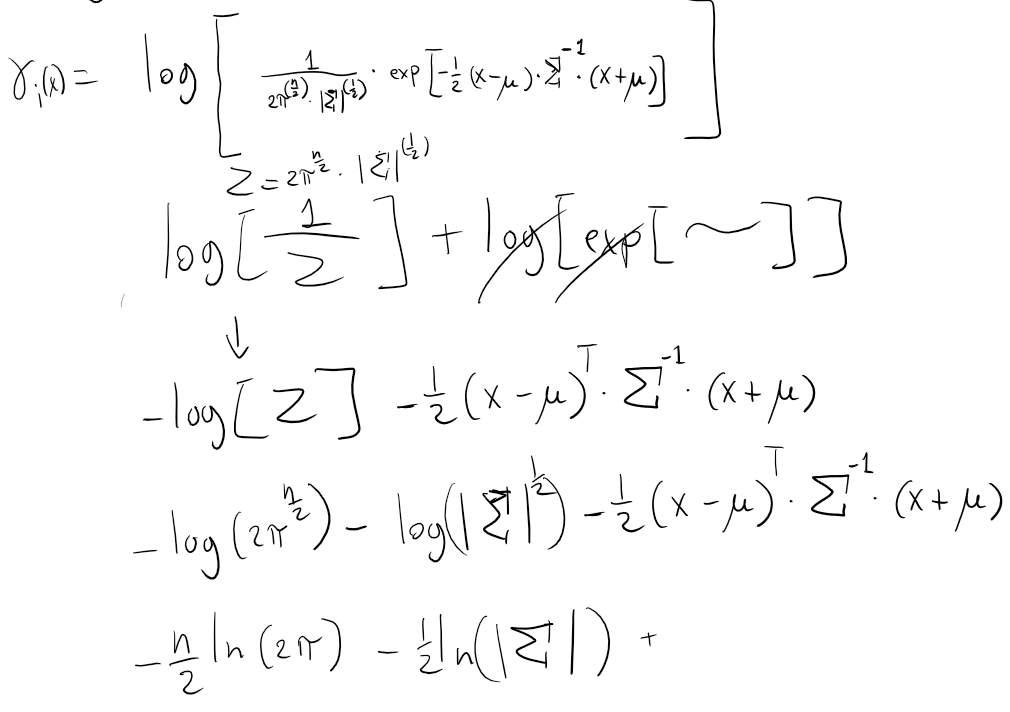
Apply the posterior probability definition as before and the log trick:

This is true for both gamma 1 and gamma 2, then we remember that gamma is defined as , so we can rewrite::

grouping together similar terms:

Prerequisite for Gaussian Likelihood: Gaussian Density §

Probability density function §

Is a non negative function that fulfills the condition:

Expected value of a scalar function §

We define the expected value of a scalar function for some probability density function :

If assumes values only on a discrete set , the expected value is:

Univariate Gaussian Density §

The univariate gaussian function (or univariate normal density) is a probability density function defined by:

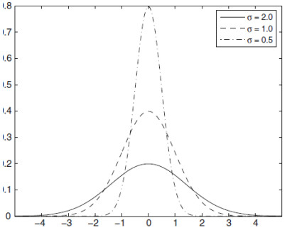
where is the expected value (or mean) of defined by:

And where is the variance defined as follows:

Now we introduce one thing that we need:

Kurtosis §

The Kurtosis is defined as a:

We are interested because, in the gaussian distribution, the Kurtosis is always 3.

The Kurtosis is the simplest way (but the noisiest) to assess if a distribution is a gaussian.

Property of the Gaussian Density §

We are interested in the gaussian density because is fully characterized by the mean and the variance and very often is indicated on papers as:

The Gaussian density is very important because:

• The aggregate effect of the sum of large number of independent random variables leads to a normal distribution.

Since the patterns can be considered as ideal prototypes corrupted by a large number of random noise, then the Gaussian is a quite good model to represent the probability distribution of the patterns.

Multivariate Gaussian Density §

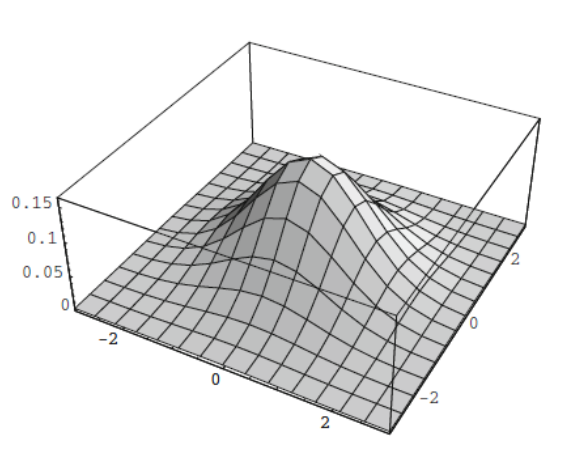
Definition of Multivariate Gaussian Density: Let (simplicity it is written ) be a vector with components, . The multivariate gaussian density is defined as:

Let’s unpack this equation:

• The left term is a fraction
  • at the denominator we have the determinant of the covariance matrix
• The right is an exponential with an argument.
  • is the mean vector, similarly defined as in univariate gaussian density. The difference is if we have 10 components i.e 10 variables, we will have a vector with 10 values that represents the mean.
  • is the covariance matrix, the equivalent in multiple dimension of the variance.

mean vector: is given by .

Covariance Matrix §

The covariance matrix is given by:

Properties of :

• Is always symmetric:
• Positive semidefinite, that is all its eigenvalues are nonnegative ()

If is the ith component of , is the ith component of and is the -th component of the covariance matrix:

• the expectation operator computed on

The last value is also called the covariance between and .

Property 2: if and are statistically independent, the covariance must be null i.e (or close to zero in real data). This is the first thing you look at when you tran a model and want to do analysis of the features. If , and are strongly correlated so they have the same information content, and you could possibly discard one of them. (not every feature holds informative contents about the data).

Eliminating redundant features lead to simpler models. Ofc you can’t eliminate both otherwise you lose the information.

Related topic: The Curse of Dimensionality

Proof of covariance matrix is always semidefinite §

Semidefinite positive means that for any column vector holds the following property: .

If is a covariance matrix then exists a column vector such that: .

For the linearity of the expectation operator, we substitute into the expression and we have that:

• where

, the product of . A term raised to two is always positive, therefore we have that .

The expectation operator on is always not null.

Mahalanobis distance §

• Mahalanobis distance, euclidean distance

Defined as:

When , then the Mahalanobis distance is equal to the euclidean distance.

Discriminant Functions for Gaussian Likelihood §

In this section we investigate the discriminant functions in the special case that the likelihood assume a normal distribution.

Recall that Discriminant Functions can be equal to posterior probability. This is shown in Equivalence between discriminant function and bayesian rule section.

So we rewrite again the equation of the log-discriminant function:

Suppose that has a normal distribution: .

Plug Multivariate Gaussian Density equation into to obtain:

Discriminant Funtions for Gaussian Likelihood equation 1 - Full passages §

Discriminant Functions for Gaussian Likelihood - General Formula §

This formula will be often referred in the specific cases that follows.

Case 1: Features are Statistically Independent §

When the features are statistically independent, the non-diagonal elements of the covariance matrix :

assumption: assume for simplicity that each feature has the same variance . This means that all patterns falls into an hyperspherical clusters of equal size.

Under this further condition, , where is the identity matrix.

• Inverse of Cov matrix:
• Determinant of Cov matrix:

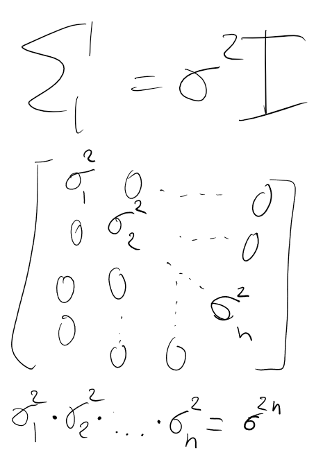Substitute these terms into the General Formula to obtain:

Some comments:

• when corresponds to the identity matrix, the Mahalanobis distance becomes euclidean distance, as we can see in
• can be simplified
• becomes

Notice that doesn’t depend from the class so it i futher simplified into:

Formula 1: Statistical Independent Features §

Case 1.1 - Statistically Independent Features, Prior Probabilities are all equal §

Recall Bayes Theorem that prior probability is , and it is the probability for each class. If it is the same, it becomes a constant therefore the formula becomes:

Formula 1.1 - Statistically Independent Features, Prior Probabilities all equal - Minimum Distance Classifier §

Definition: this is called minimum-distance classifier and apply the minimum-distance rule (i.e K-Means). The mean vector (called centroid in the K-means), is also viewed as a prototype for a pattern belonging to the class

Case 1.2 - Statistically Independent Features, Prior probabilities not all equal §

If the prior probabilities are not all the same, the decision is influenced in favor of the class with the highest apriori probability.

In particular, if a pattern has the same distance from two or more different mean vectors, the decision rule chooses the class that has the highest a priori probability.

Consider the Formula 1 Statistical Independent Features

Using properties of the inner product, it can be rewritten as:

Apply the following simplifications:

• is the norm of
• is the norm of
• is equal to since So we can rewrite it as:

Since is the same for all , it is a constant. Therefore it can be neglected:

That is a linear expression of the following form:

is often called threshold or bias for the th class.

This is called linear discriminant function or linear classifier

Formula 1.2 - Statistically Independent Features, Prior Probabilities NOT all equal - Linear Classifier §

Of the form:

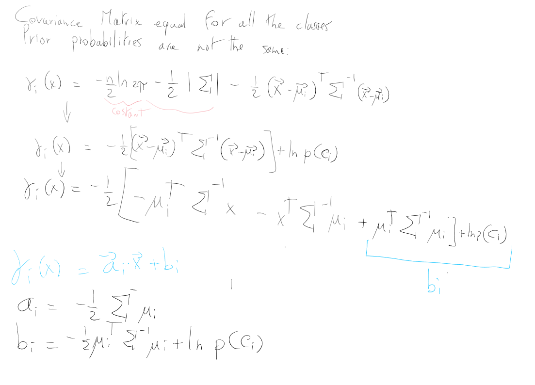
Case 2: Covariance Matrix is the Same For All Classes §

This corresponds to the situation in which the patterns fall in hyperellipsoidal clusters of equal size.

Consider Discriminant Functions for Gaussian Likelihood - General Formula

Since the first two tersm are independent of (cov matrix is the same for every class, therefore a constant), they can be neglected and becomes

Formula 2 - Covariance Matrix Same For All Classes, General Formula §

Case 2.1 Covariance Matrix Same for all Classes, Prior probability are all equals §

The last term be neglected. Thee minimum mahalanobis distance rule, where to classify a pattern we compute the m. distance between and each vector and assign the pattern to the class whose mean is closest. A classifier that apply this rule is called minimum mahalanobis distance classifier.

Formula 2.1 Covariance Matrix Same for all Classes, Prior probability are all equals §

If the prior probabilities are not all the same, the decision is influenced in favor of the class with the highest a priori probability. In particular, if a pattern x has the same distance from two or more different mean vectors, the decision rule choose the class that has the largest a priori probability. Similar to Case 1.1 - Statistically Independent Features, Prior Probabilities are all equal.

Case 2.2 Covariance Matrix Same for all Classes, Prior Probability NOT are all equals §

Consider Formula 2 - Covariance Matrix Same For All Classes, General Formula

The term does not depends by the index and it can be considered an additive constant that can be neglected.

Hence the discriminant functions are:

Also in this case the discriminant function are linear. The resulting decision surface between two adjacent region and is again an hyperplane, unlike the case of features that are statistically independent, are not generally orthogonal to the line that joins the mean and .

Here’s the passages to distinguish from

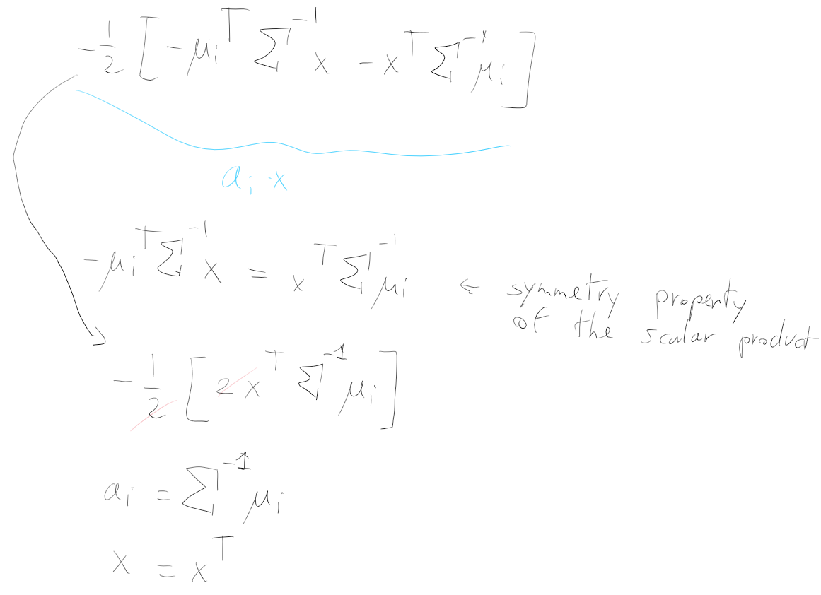
Formula 2.2 Covariance Matrix Same for all Classes, Prior Probability NOT are all equals §

Of the form:

Case 3 - Covariance Matrix Is Not The Same for All Classes §

The most general case that you can find in real data.

Consider again: Discriminant Functions for Gaussian Likelihood - General Formula

Formula 3, Covariance Matrix Not The Same For all Classes §

Notice that the unique term that is an additive constant is . Drop it to obtain:

where:

The discriminant functions in this case are nonlinear. In particular, in the binary classifiers the decision surfaces are hyperquadrics.

The results obtainted for the binary classifiers can be extended to the case of more than two classes, fixed that are two classes that share the decision surface.

Optimality: a linear classifier is optimal only when Case 2 Covariance Matrix is the Same For All Classes.

Summary table - Discriminant functions for gaussian likelihood §

	Name	Formula	Alternative form	Alternative name
Formula 0	General Formula
Formula 1	Statistical Independent Features
Formula 1.1	Statistical Independent Features, all equal prior probabilities			Minimum distance rule/classifier
Formula 1.2	Statistical Independent Features, NOT all equal prior probabilities			Linear
Formula 2	Covariance Matrix Same for all classes
Formula 2.1	Covariance Matrix Same for all classes, Prior probability are all equals			minimum mahalanobis distance rule
Formula 2.2	Covariance Matrix Same for all classes, Prior probability NOT are all equals
Formula 3	Covariance Matrix is not the same for all classes