Gradient Descent (GD) and variants (momentum, ADAM, stochastic)

---

Gradient Descent (GD) §

• SC - Lezione 16 - Gradient Descent Methods, with momentum, ADAM, Stochastic, Levenberg-Marquad
• ML - Lezione 8 - Error Backpropagation for Feed-Forward Networks / ML2 - Lecture 9.1 - Error Back Propagation
• CV - Lab - Optimization, Gradient Descent and variants

Gradient Descent introduction §

The gradient descent is an iterative method for mathematical optimization. Idea: take repeated steps in the opposite direction of the gradient (or approximate gradient) of the function at the current point, because this is the direction of steepest descent.

In Machine Learning, this method is used to minimize the loss function.

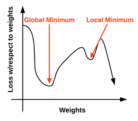
Gradient Descent Analogy (from wikipedia) §

Imagine some people are stuck in the mountain and are trying to get down (find the global minimum). Since there is heavy fog, they must use local information to get down (find the minimum). They can use the gradient descent by looking at the steepness (slope/gradient of a line) of the hill at their current position, then proceeding in the direction of the steeping descent (i.e. downhill). Using this method they will eventually get down or get stuck in some hole (local minimum), like a mountain lake.

Assume also that they have sophisticated instruments to take measurements (differentiation of a function), and they must get down before sunset. Taking measures requires time, so they should minimize their use of the instrument if they want to get down in time. The difficulty is choosing the frequency (learning rate) at which they should measure the steepness of the hill. The amount of time they travel before taking another measurement is the step size.

Standard Gradient Descent - Definition §

Consider a neural network for illustrate the concept, let be a linear combinations of its input and current parameters (weights and bias ): . Let the loss function be the sum of squared error for a single data point : .

Descent Mechanism it is done in two steps.

In the first step, we compute the gradient, that tells us how much change in any parameter affects the error functions. We compute the partial derivative of the error function with respect to a specific weight :

Using the chain rule (from calculus), the partial derivative with respect to a weight connecting connecting input to output is:

In the second step, we update the weights by taking a step in the direction opposite to the gradient (downhill):

• are the updated weights and are the old weights.
• is called learning rate and will be described in the next section.

This update is performed iteratively, eventually leading the model’s parameters to a minimum point in the error landscape.

Learning Rate §

It is important because the limitation of learning descent helped to developed variations of gradient descent that have an impact in the learning of deep learning models.

In learning of machine learning models, this is an hyperparameter. Often denoted with or .

• Large : The steps are too big. The algorithm might overshoot the minimum and bounce around chaotically, failing to converge.
• Small : The steps are very small. The algorithm will take too long to reach the minimum, making training inefficient.
• Just Right : The steps are balanced, allowing the algorithm to quickly and efficiently settle into the minimum.

Convergence and epochs §

The two steps described above are repeated iteratively for hundreds or thoudsnds of epochs (full passes through the training data), until the parameters converge.

Convergence means that applying again the gradient descent the steps become negligibly small, because the algorithm has reached the bottom of the valley (minimum error).

Speed of convergence §

Theoretically speaking, when we choose an error function it must be convex. Being convex guarantee that it is differentiable and then we can apply the derivative.

If a function is convex, the Hessian matrix (i.e the matrix containing all the partial second derivatives of a function) is symmetric and positive.

The Hessian matrix has an important property: the eigenvalues of the Hessian matrix determine the actual speed of convergence of the GD method. This is expressed by the ratio:

• is the minimum eigenvalue and is the maximum eigenvalue.

The Hessian describes the curvature of the function (since it’s the matrix of the second partial derivatives, and in a single parameter function the curvature is described by the second derivative).

If , then the function has very different curvatures in different directions, which can slow the convergence of the GD method.

Gradient Descent with momentum (GDM) §

Visualizing gradient descent method shows that using a constant learning rate lead to a zig-zag pattern (oscillation), especially in narrow valleys of the error surface. This inefficient bouncing slows down convergece.

To mitigate this, we can add momentum. Instead of calculating the step based solely on the current gradient, we maintain a velocity vector that accumulates the history of past gradients.

The velocity vector (or accumulated gradient) is defined at step :

• is a hyperparameter with values between 0 and 1. It determines how much of the past history we keep.
• is the velocity vector from previou step .

Then we update the weights:

Why it works: momentum acts like a physical mass rolling down a hill:

• Smoothing. if the gradient zig-zags (oscillates positive and negative); the sum of these opposing gradients in the history tends to cancel out, reducing the side-to-side motion.
• Acceleration: instead, if the gradient consistenly points in the same direction, grows larger, effectively increasing the step size and speeding up convergence along flat sections.

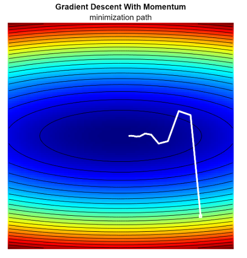As conseguence, this lead to faster convergence.

ADAM - Adaptive Moment Estimation §

ADAM is an improvement of GDM, that combines momentum with RMSProp (second moment). It adapts the learning rate individually for each parameter.

The first momentum is computed like in the previous section:

The second momentum:

• means squaring each element of the gradient vectory individually

Like before, and are hyperparameters, with values between 0 and 1 that controls how much of the previous momentums influences the current update.

The update step combines both moments:

• A small is added to avoid dividing by zero.

Why it works:

• (numerator) like GMD provides momentum to smooth the path
• (denominator): scales the learning rate:
  • If gradients are large/noisy (high ), the step size automatically shrinks (stable)
  • If gradients are small/sparse (low ), the step size increases (faster)

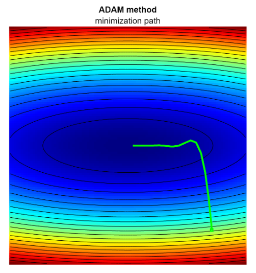
ADAM effectively adapts the learning rate by normalizing the update using the moving average of the squared gradients ().

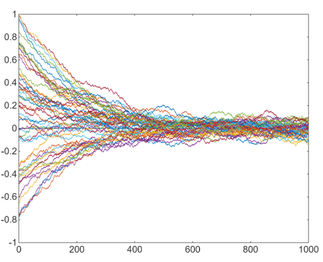
Stochastic Gradient Descent (SGD) §

Idea: When dealing with very large datasets, computing the gradient of the error function over the entire dataset is computationally prohibitive. SGD addresses this by updating the model’s parameters using only a single sample (or a small subset) at a time.

• Trade-off: this approach introduces noise, as a small sample only provides an approximation of the true gradient.
• Benefit: despite the noise, SGD often leads to faster convergence for large datasets because parameters are updated much more frequently. The noise can also help escape shallow local minima.

Pure vs Mini-Batch:

• Pure SGD: selects one single data point, computes the gradient, and updates weights. (High noise, very fast updates).
• Mini-Batch SGD: uses a small subset of data points (a batch) to compute the gradient.

Mini-Batch SGD is the standard approach in modern Deep Learning because it balances computational efficiency (vectorization) with gradient stability.

Formal Definition (Mini-Batch): Let be the loss function for a single data point. Consider a mini-batch of size :

The update rule is:

where is the gradient computed over the subset.

In practice, we often divide this sum by (compute the average) to keep the gradient scale independent of the batch size.

Convergence in SGD: Because we are processing data in chunks, we need to define the training cycles:

• Mini-batch size (p): the number of samples processed in one go.
• Iteration: one single update step (one forward/backward pass of a batch)
• Epoch: One complete pass through the entire dataset

If a dataset has samples and the batch size is : Training Loop: usually, the dataset is shuffled, and then a loop runs through the data in chunks of size . Once the loop finishes (all data seen), one epoch is complete. This is repeated for many epochs (often thousands) until the loss converges.

Sampling Strategies:

• Without Replacement (Standard): The dataset is shuffled, and we partition it into batches. Each data point is selected exactly once per epoch.
• With Replacement: For every batch, we randomly sample points from the full dataset. The same data point could be chose multiple times in one epoch, while others might be skipped entirely.

Usually, without replacement is preferred. It ensures the model sees every single data point equally, making more efficient use of the data, improving convergence stability, and reducing variance.

---

Gradient Descent Vs Backpropagation §

• Gradient Descent is the strategy of optimization of a function, in the context of neural networks it is used to minimize the Loss function.
• Backpropagation is an algorithim techniques used exclusively within neural networks to compute the gradient required by Gradient Descent. It uses the chain rule from calculus. In short it works in two phases:
  • in the forward pass (the prediction), data is passed forward through the network layer by layer, an output prediction is generated and the loss is calculated comparing the output to the true target.
  • In the backward pass (error attribution), starting from the output layer, the error is calculated and propagated backward through the network. At each layer, backpropagation efficiently computes the contribution of each weight to the final error by applying the chain rule.

Backpropagation provides Gradient Descent with the value of the graident.