NLP - Lecture - Vector Space Models
When we consider vector we talk about vector space models.
So what are meaning? We aim to arrive to vector representation that make it possible to distinguish between different situations.
- Where are you heading?
- Where are you from?
Even if they share a lot of words the meaning is completely different
Consider two questions what is your age and how old are you? they have the same meaning
Vector space models may help to:
- identify whether the first or second pair of questions are similar in meaning even if they do no tshare the same words
- Identify similarity for a question answering, and summarization
- Allow capturing dependencies between words
Vector Space Models Applications For instance ”you eat cereal from a bowl”, words cereal and bowl are related. You buy something and someone else sells it: the second half of the sentence is dependent on the first half.
Vectors-based models capute these and many other types of relationships among different sets of words.
Distributional Hypothesis
“You shall know a word by the company it keeps.”
Vector space models:
- Represent words and documents as vectors
- Representation that captures relative meaning by identifying the context around each word in the test -> this captures the relative meaning
Observation: words that are synonyms tend to occur in the same environment, with the amount of meaning difference between words “corresponding roughly to the amount of difference in their environment”
Example: Ongchoi
What does ongchoi mean? This is a chinese word.
Suppose you see these sentences:
- Ongchoi is delicious sautéed with garlic
- Ongchoi is superb over rice
- Ongchoi leaves with salty sauces
And you’ve also seen these:
- spinach sautéed with garlic over rice
- Chard stems and leaves are delicious
- Collard greens and other saultes
So this suggests that Ongchoi is a leafy green like spinash, chard, or collard greens. Since the words of the context and other leafy green are the same. In fact Ongchoi is a Leafy Green.
Word by Doc and Word by Word
To capture relations by words we can use two approaches:
- word by document
- word by word
Co-occurence Matrix
If i have to compute some vector or distributional models, i have to verify the occurence of words with other words in a collection. So the idea is to build this co-occurence matrix.
Depending on the task at hand, several possible designs exist.
Each row represent a word in the vocabulary and each column represent how often each word in the vocabulary appears nearby. Vectors can be constructed from the co-occurence matrix.
Word by Document Design
Number of times a word occurs within a certain category
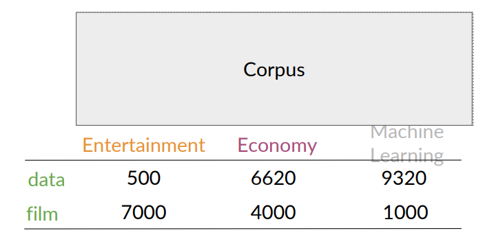 For instance, entertainment category vector is
Each document is represented as a vector of words.
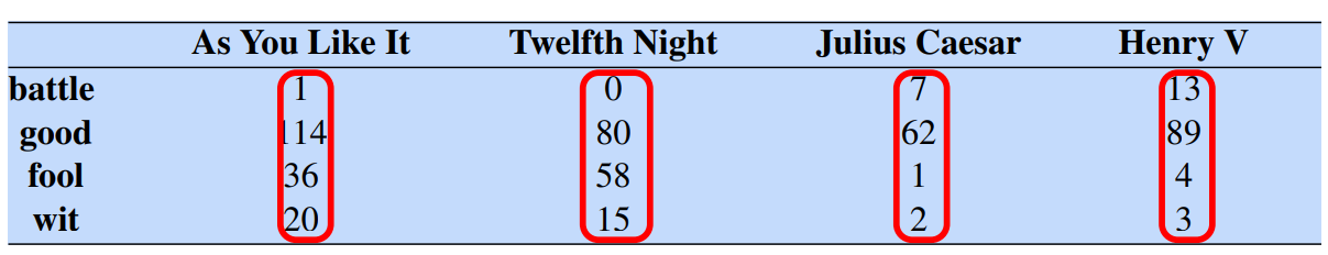
Vectors are the basis of information retrieval. As we can see, vectors are similar for two comedies, but comedies are different than the other two.
A vector space is a collection of vectors, and is characterized by its dimension.
Comedies have more word like fool and wit, and fewer battle.
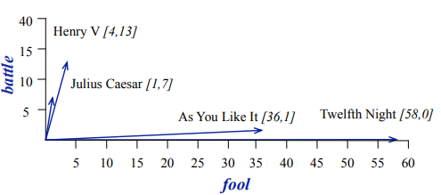
- Battle is “the kind of word that occurs in Julius Caesar and Henry V”
- Fool is “the kind of word that occurs in comedies, especially Twlefh Night”
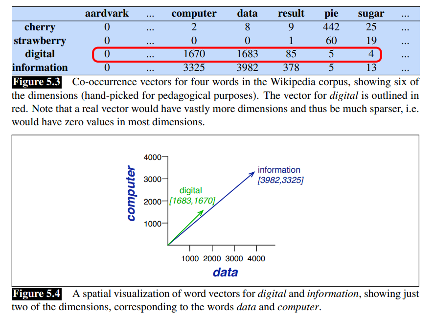
The co-occurrence of two different words is the number of times that they appear in a corpus together within a given word distance
Assume that you are trying to construct a vector that will represent a certain word.
Create a matrix where each row and column corresponds to a word in the vocabulary
Keep track of number of times they occur together within a certain distance
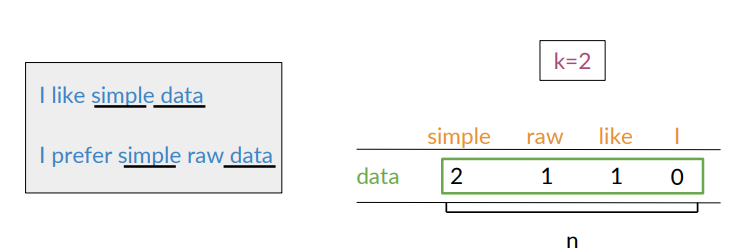
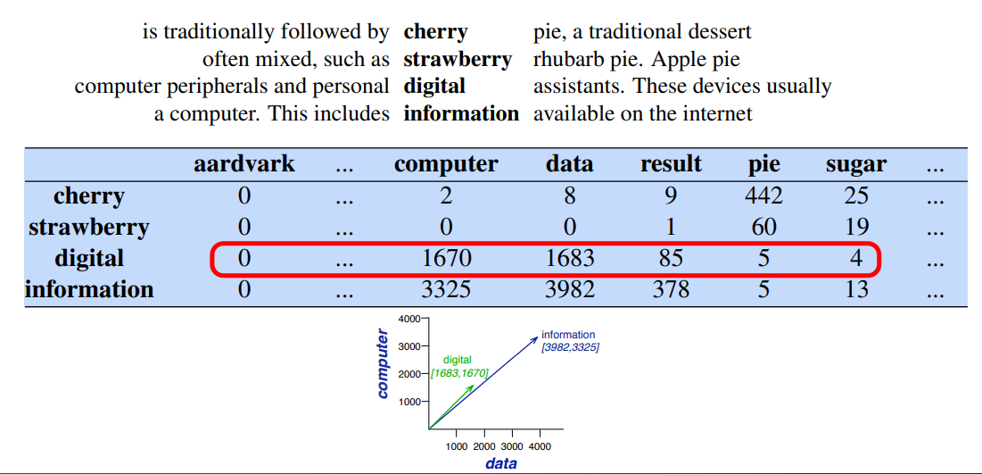
Word-Word Matrix
Two words are similar in meaning if their context vectors are similar.
Vector Space
A representation of the words data and film is taken from the rows of the table Alternatively, the representation for every category of documents could be taken from the columns.
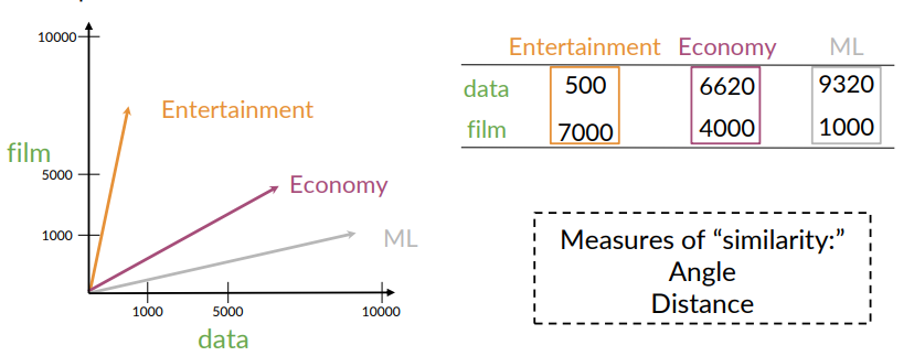
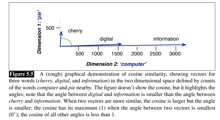
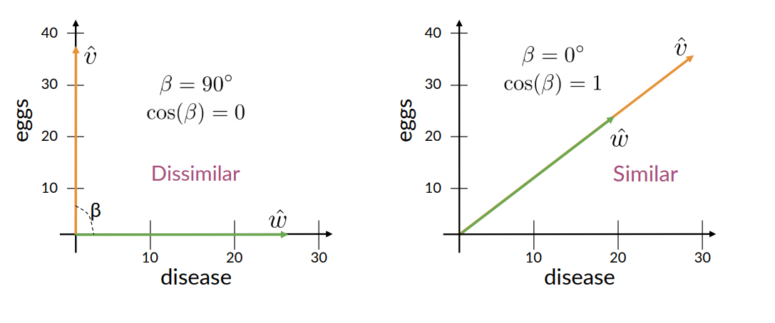
Comparing Vectors
One way to measure similarity is through cosine similarity is defined as:
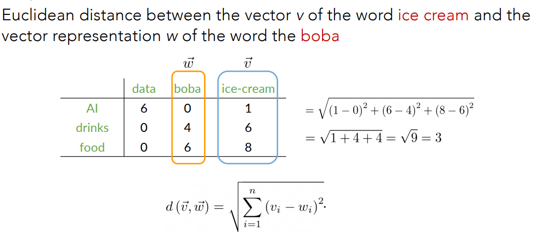
Another way is to use the euclidean distance.
Consider two corpus “A” on Entertainment and “B” on Machine Learning.
Euclidean Distance:
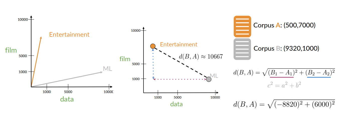
- Intuition: in the second figure, it’s simply the lenght of the line that connect these two points.
Example:
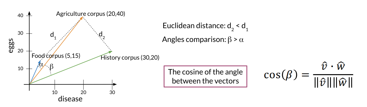
But Euclidean distance is not always accurate, for instance when comparing large documents to smaller ones.
In this case it’s better to use cosine similarity
Raw Frequency is not the best representation
However, the co-occurence matrices we have seen represent each cell by word frequencies.
Frequency is useful i.e If “sugar” appears a lot near “apricot”, that’s useful information.
But overly frequent words like “the”,“it”, or “they” are not very informative about the context. They do more information about grammar than semantics.
It’s a paradox: How can we balance these two conflicting constraints (words very frequent but useless to extract meaning)?
Two common solution.
TF-IDF
The first method is TF-IDF:
- tf-idf value for word
in document
TF-IDF: Term Frequency
Term Frequency (TF) measures how frequenty a term
In this way, a word appearing 100 times in a document doesn’t make that word 100 times more likely to be relevant to the meaning of the document.
TF-IDF: Document Frequency
Document Frequency (DF) is the number of documents in which the term
Collection Frequency vs Document Frequency
Collection Frequency sums all occurencies of the term across all documents. Document Frequency instead is the number of time the term
occurs all documents.
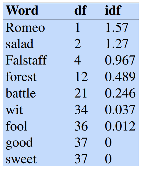
Example: Collection Frequency vs Document Frequency
- Using collection frequency on words “Romeo” and “action” over the Shakespeare corpus lead to different result thant document frequency.
- “Romeo” is a peculiar word that appears in only one document.
- “Action” is a more common word that appears in various Shakespeare plays

We consider the inverse document frequency (IDF) computed as:
is the total number of documents in the collection. for the Shakespeare collection. - IDF reduces the weight of frequent (less informative) terms and increases the weights of the rarer one (more informative).
Final tf-idf weighted value for a word
Now, by multiplying Term Frequency by Inverse Document Frequency we obtain the final TF-IDF value.
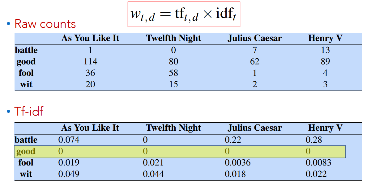 Consider the word “good”, it appears in every document, so
In other words, frequent words have no discriminative power and so tend to have a lesser value.
What is a document? Could be a play or a Wikipedia article. For the tf-idf, documents can be anything. We often call each paragraph a document.
Pointwise Mutual Information
For Word-By-Word matrix we can use the Pointwise mutual information defined as:
PMI measures how much more often two words co-occur than we would expect if they were independent.
It answers the question “do events
It compares the joint probability
If the two words are independent then
- Positive PMI means the words co-occur more often than expected;
- Negative PMI means they co-occur less.
The formula as is written ranges from
For example consider two words
To handle this, we just replace negative PMI values with 0.
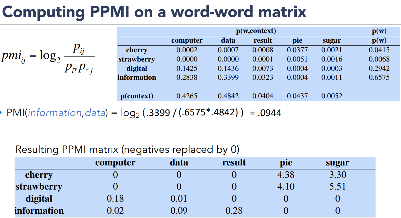
Positive PMI (PPMI) between two words is:
Let’s see an example of computing PPMI on a word-word matrix.
Matrix
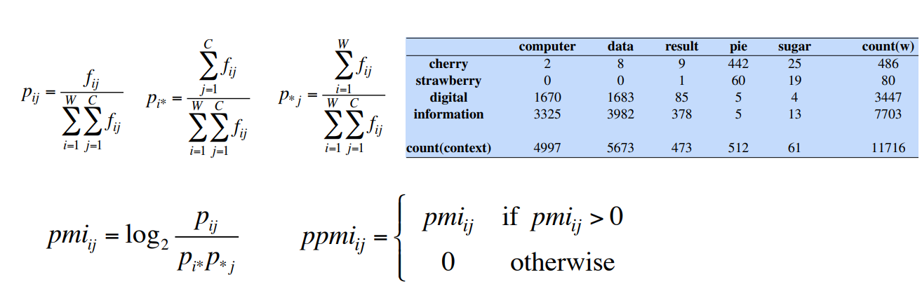
- In the columns i have the context words
- In the rows i have the words for which i want to compute the PPMI
- I also count words and context words for computing the probabilities.
In this way i’m able to compute the joint probability and marginal probability.
Then i can compute
Examples:
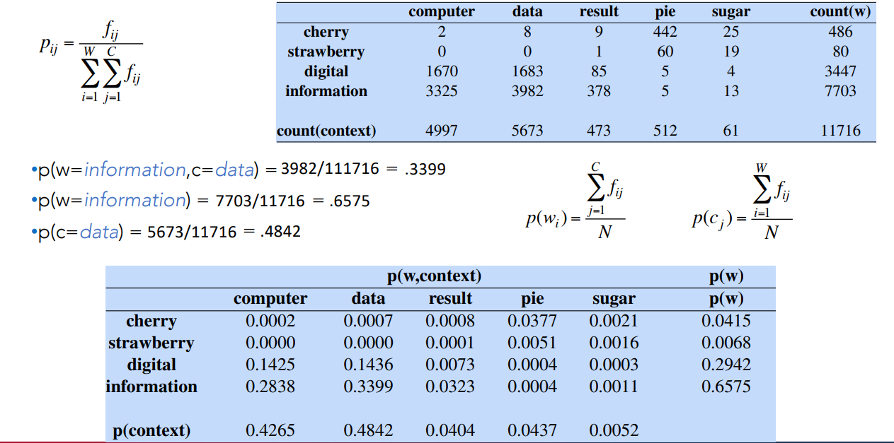 The matrix on the low part is the matrix of the probability of each word with each context word.
These are the words vectors.
PMI Drawbacks
The Problem with PMI is that is biased toward infrequent events i.e very rare words have very high PMI values. This happens because the denominator
Two solutions:
- Give rare words slightly higher probabilities
- Use add-one smoothing (which has a similar effect)
To implement the first idea, it is possible to raise the context probabilities to an
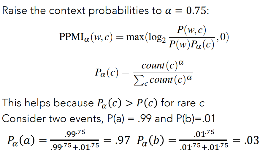 We simply replace
The example clarify: if i consider the word
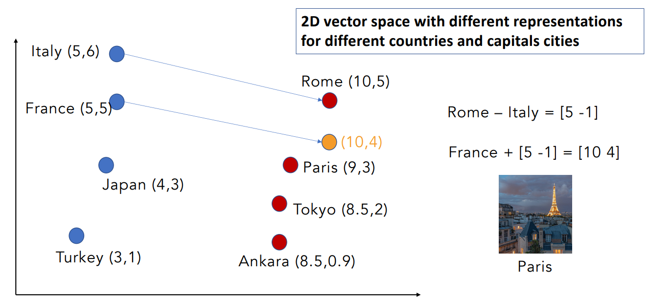
Manipulating Words in Vector Spaces
Suppose we have a vector space with countries and their capital cities
- We know that Rome is the capital of Italy
- We don’t know the capital of France
Goal: infer the capital of France by the known relationship.
Word vectors can be used to extract patterns and identify certain structures in our text.
Example
- One can use the word vector for France, Italy, and Rome to compute a vector that would be very similar to Paris.
- Then use the cosine similarity of the vector with all the other word vectors and find that the vector of Paris is the closest.
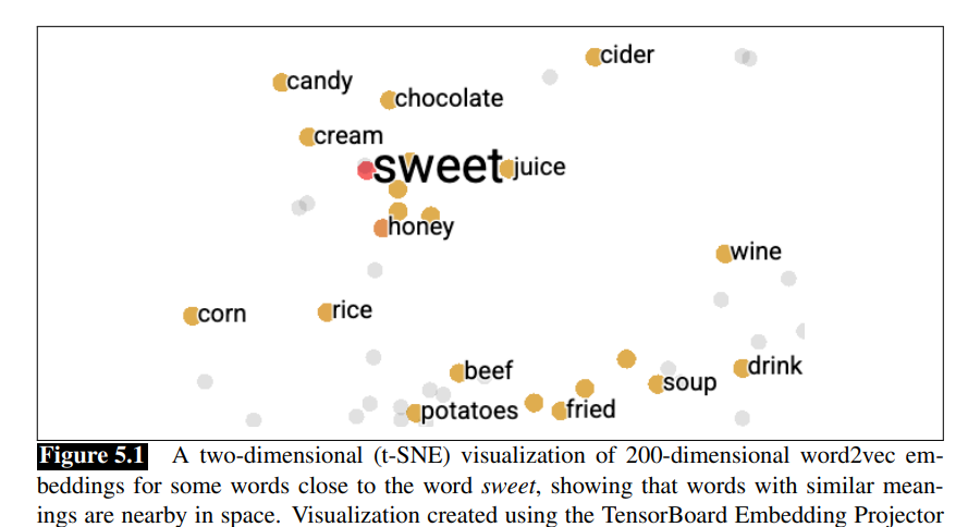
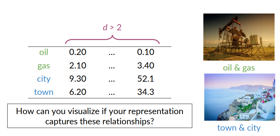
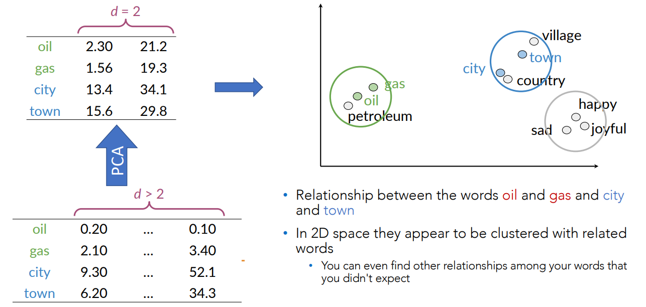
With vectors of very high dimensions PCA (or other dimensionality reduction techniques) can be used to plot vectors in 2D or 3D spaces.
t-Distributed Stochastic Neighbor Embedding(t-SNE)
It belongs to a class of visualization algorithms called manifold learning. An unsupervised, randomized algorithm, used only for visualization.
Applies a non-linear dimensionality reduction technique where the focus is on keeping the very similar data points close together in lower-dimensional space.
Preserves the local structure of the data using student t-distribution to compute the similarity between two points in lower-dimensional space.
Used for visualization purposes because it exploits the local relationships between data points and can subsequently capture nonlinear structures in the data.
t-SNE isn’t like PCA and whatever you add new data points you need to recompute it entairly.
In the next lesson we will see dense word vectors, and we will use a neural network that compute the word vectors and we will see its called word embeddings.