SC - Lezione 18
Checklist
Domande, Keyword e Vocabulary
- Netflix prediction matrix problem
- Application of SVD + Gradient Descent minimization problem
- Why we use the SVD
- Choose of the parameter K
- Rating Prediction
- Incomplete SVD (also called SVD based on stochastic gradient descent)
- Page Rank
- Source-node i vs target-node j convention
- Source-node j vs target-node i convention
- Property of Adjacency Matrix and Number of paths
- Scaled Adjacency Matrix
- Importance of a page
- Nonlinear system
- Stochastic respect to the columns
Appunti SC - Lezione 18 - Netflix Prediction Matrix Problem using SVD and Gradient Descent
Netflix Prediction Matrix Problem
In this application we use both the SVD and the gradient descent minimization problem
Problem Formulation
We have a movie recommendation system.
A matrix
We represent the set of users ad
Important: If an user has not ranked a movie, the value is left empty or at a specific default value.
We want to build a recomendation system that predict the missing entries. We call the predicted matrix as
This new matrix will have a rank
: in this context, is a and its rows are the unscaled components of the users in a space of dimension , whose basis vectors are the rows of : it’s simply the diagonal matrix with the singular values on the diagonal
: it’s a matrix and its columns are the unscaled components of the movies in the subspace of dimension spanned by the columns of
The parameter k: if k is too large then the model may suffer from overfitting, if k is too small it may not able to capture the complexity of data.
Rating Prediction
After computing the SVD we have our prediction matrix
Example: the predicted rating of movie
We don’t know what are
To address this issue, a technique called incomplete SVD or SVD based on stochastic gradient descent is used.
We want to compute
Incomplete SVD Method
Steps of the Algorithm
- Initialize matrices
, and with small random values - Minimize the prediction errors until you reach a convergence point or after a predetermined number of step
Minimization steps:
- Select a random set of known entries of the matrix
- For each known entry
compute the prediction using the current matrices , , by doing the scalar product of and thus recaving a prediction matrix - Compute the difference between
and and this is called the prediction error - Update the matrices
, and to reduce the prediction error, or more generally to minimize an objective function related to prediction errors using Gradient Descent (Or Stochastic Gradient Descent)
Objective Function to minimize
The objective function depends on the two matrices:
The objective function to minimize:
- the (i,j) under the summation is a subset of the (i,j) of the known
matrix. is a regularization parameter is the row of : (note it’s not u[i]butu[i,:])is the column of (note it’s not v[j]butv[:,j])
The summation contains 2 terms:
- the 2-norm square of the error that is:
- the 2-norm square of
and the 2 norm square of : multiplied by a regularization parameter
Once the matrices
We will use the GD descent so we will need to compute the gradient. The derivative i.e the gradient will be computed respect to te three variables:
Gradient Computation: Recall: Gradient Descent Method.
We need to compute the gradient of the objective function
- The gradient of
respect to the entries is: - The gradient of
respect to the entires is:
Then i have to update
- update
- update
Note: In our example we compute the three matrices and then multiply them together in order to get the predicted matrix. In other application we do the reverse process: we compute the 3 matrices using a matrix we already have.
Page Rank
The PageRank algorithm evaluates the importance of web pages based on the link structure of the web.
It operates on the principle that a page is important if it is linked to by other important pages.
The algorithm assigns a numerical weight (score) to each element of a hyperlinked set of documents with the purpose of measuring its relative importance within the set.
Relevance vs Importance
- Relevance: how well a web page matches a user’s search query, evaluated through factors like keyword alignment, content quality, and contextual signals.
- Importance: web page authority or trustworthiness, evaluated by the quantity and quality of incoming links (backlinks)
PageRank evaluates the importance of web pages based solely on the web’s link structure, without considering the content.
Problem Formulation - Direct Graph
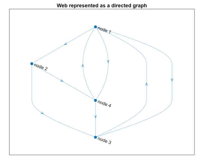
A web consists of web pages and links among them. Therefore it is a directed graph where pages are nodes and links are edges.
Adjacency Matrix
Using the i- target j convention, we define the adjacency matrix. Since this is a linear algebra problem we want an adjacency matrix to manage the data.
We eventually transpose this to have a source-node j vs target-node i convention
Recap the two convention:
=source node i vs target-node j convention, source-node j vs target-node i, convention
The entry
Property of an adjacency Matrix: An adjacency matrix is always square and usually sparse, and can be defined as a Matlab sparse-format matrix.
In the source-node j vs target-node i convention, we have that sparse matrix have an interesting property. A non-zero entry in row
For instance consider this:
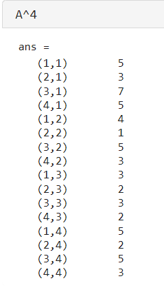 There are 7 paths of length 4 from node 1 to 3.
There are 5 paths of length 4 from node 4 to 1.
There are 7 paths of length 4 from node 1 to 3.
There are 5 paths of length 4 from node 4 to 1.
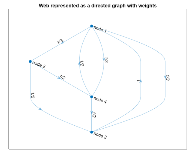
Penalizing nodes with a too much high number of outgoing links: Scaled Adjacency Matrix
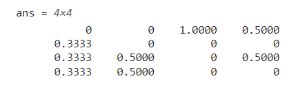
We want to penalize nodes with an high number of outgoing links, and for doing this we apply a normalization respect to the total number of outgoing links from that node:
In doing this we obtain the scaled adjacency matrix of the web.
Importance of a page
The importance of node
Since
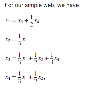
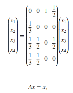
This is not a linear system
This isn’t a linear system because a linear system require that you have a known vector i.e
Here we have that
We saw the definition of eigenvalue/egeinvectors as:
Stochastic respect to the column
Recall that we already encountered the concept of stochastic matrix when we applied the power method for smoothing a random polygon.
The scaled adjancecy matrix A of our web is “stochastic respect to the columns” which means that its column vectors have non negative entries and 1-norm equal to 1.
Also it has only 1 dominant eigenvalue and it is 1. And it has algebraic multiplicity = 1, so it is unique. This implies that the solution exists and it is unique to the problem
So it becomes a problem of computing the dominant eigenvector of a matrix, that is solved using the Power Method that we saw. But also specific method for sparse matrices works such as Matlab’s eigs.
An extra step we do in Matlab is that the eigenvectors are versor in 2 norm, but we can scale in any way we want these vectors, so we just normalize them such that
In real life applications there are some issues:
- The matrix could be too large for applying the power method
- The adjacency matrix may not be column-stochastic
PageRank’s approximated scaled adjacency matrix
Non column-stochasticity: a page can have dangling nodes, that are nodes without outgoing links. It can also happen that a subset of nodes can not be reachable from another subset or nodes.
So we need to approximate the matrix A with a matrix that we call
We note that for such a matrix the spectral radius is still 1, the dominant eigenvector is unique and its entries have the same sign, so they can be scaled to be all positive.
The matrix M is defined as weighted average between the scaled adjacency matrix A and a matrix S:
is the scaled adjacency matrix is a costant matrix, where each entry is is called the weight parameter. Usually set to
The dominant eigenvalue of
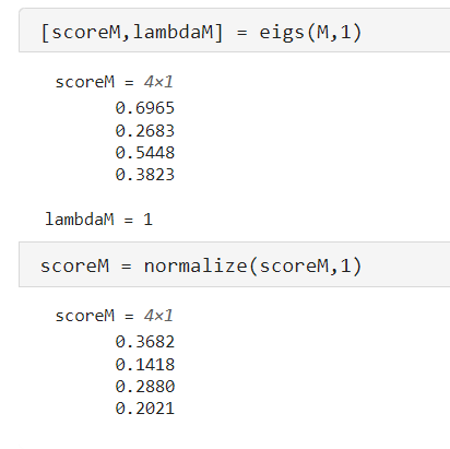 We are not interested that the numbers are the same because we want a score for each page. The important thing is that the order i.e. the first, the second most important pages, are in the same position. Another important property that we want is all the elements are strictly positive, since a negative score doesn’t have any meaning.
The Heart of PageRank Algorithm consists in computing the dominant eigenvector of the matrix
where
Observation
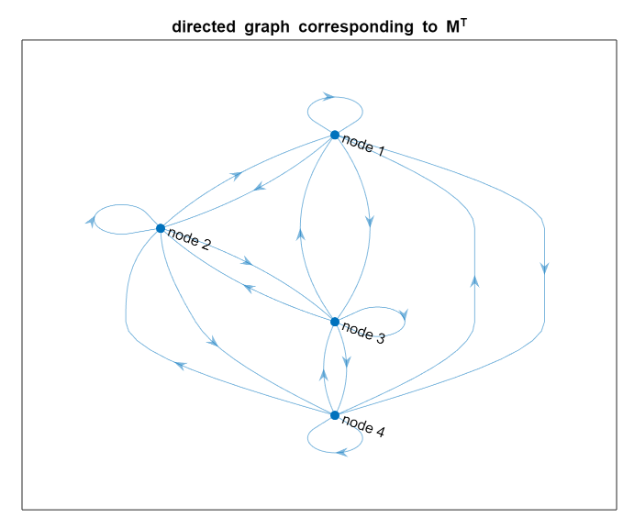 Why there are these “cappi”?
Notice that the original matrix hasn’t any cappi
Why there are these “cappi”?
Notice that the original matrix hasn’t any cappi
 and also the diagonal is zero
 We modified the matrix in a way that all the elemtens are non zero. Also, there are more edges in the newer graph because each node is connected to each other.